Hypothesis testing proportions - part 1.

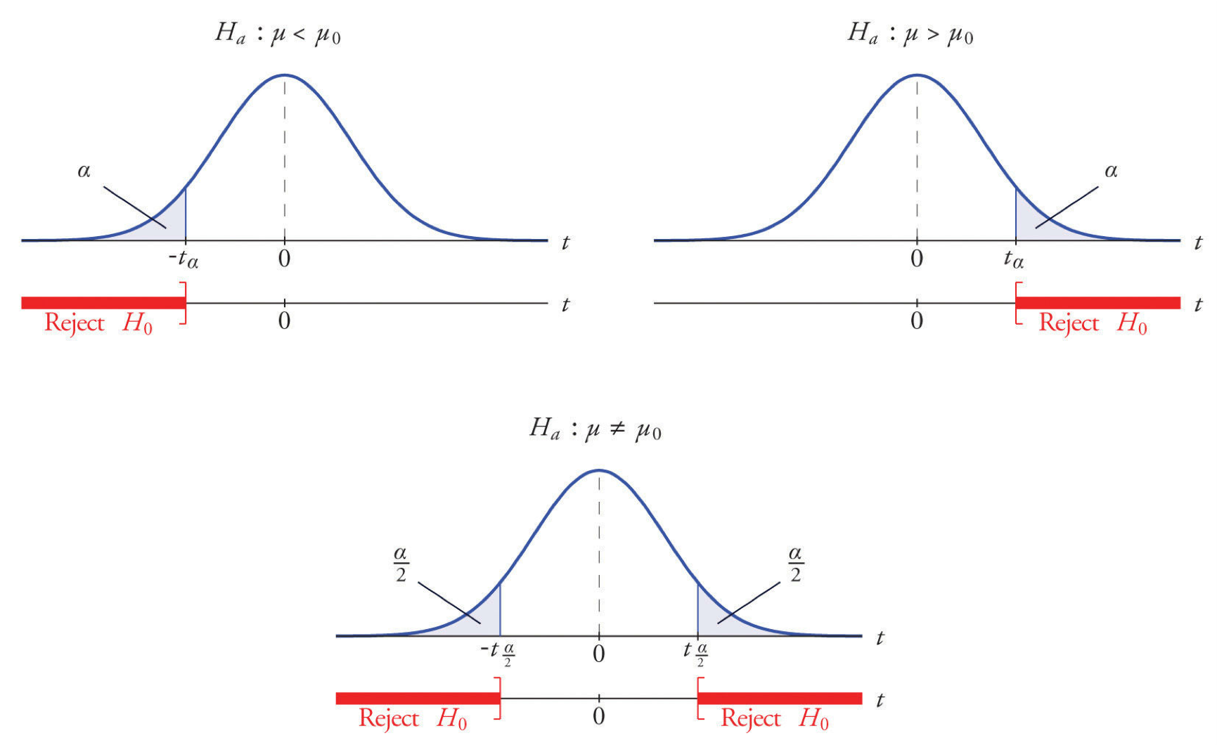Rejection regions in hypothesis testing.

In this post I examine a bit of statistical theory behind hypothesis testing using the specific case of population proportion. I’m assuming a basic background knowledge of probability and statistics.

It’s probably going to get a bit dry, but I’ll try to keep it short! In case your tolerance for theory is low:

TL;DR:

1. To test hypotheses about proportions, we can treat our sample data as Bernoulli random variables, giving us a parametric model.
2. Since the sample proportion \(\hat{p}\) is the maximum likelihood estimator for this model, we can use a Wald test.
3. If the null hypothesis is \(p = p_0\), the test statistic is \(\frac{\hat{p} - p_0}{\sqrt{\hat{p}(1 - \hat{p})/n}}\) and it is approximately normally distributed.

Suppose we have a population and two possible states of interest for members of this population. For example, the answers to a yes-or-no question on a survey, or whether a person tests postive for a disease condition. We’d like to formulate and test some hypothesis about the proportion of the population in each state.

But populations are too big. So we need to take data and infer something about the population – that is, we need to do inferential statistics. There are different paths we can take to do this, but in this article, we’ll look at the classical analytic hypothesis testing approach. Since analytic here pretty much means “derived from mathematical theory”, that’s why we need all the theory!

One way to model this situation is to represent the data by a sample of Bernoulli random variables, that is binary independent random variables \(X_1, \dots, X_n\), taking values in say \(\{0, 1\}\) with probability mass function \[\begin{aligned} P(X = 1) &= p\\ P(X = 0) &= 1-p \end{aligned}\]

where \(p\) is unknown.

Since we don’t know \(p\), we are really thinking about a family of probability distriutions, one for each \(p\). This is a statistical model, and since the family depends on the single parameter \(p\), the model is parametric.

In classical hypothesis testing, we’re actually considering two hypothesis, the so-called “null”, and “alternative”. It’s important to recognize we are only comparing these hypotheses, and the conclusion we come to after testing is to provisionally favor one or the other¹.

For population proportion, a typical null hypothesis takes the form \(p = p_0\) where \(p_0\) is some specific hypothetical value². The value \(p_0\) will often be some “conservative” choice³. The set up of the hypothesis test gives preferential status to the null – we require strong evidence to favor the alternative. A common analogy is “innocent until proven guilty”, that is, until certain high evidential standards are met.

After settling on a null hypothesis, we can formulate an alternative. For population proportion, typical possibilities are \(p \neq p_0, p \geqslant p_0\) and \(p \leqslant p_0\). For simplicity, let’s just focus on the first one, taking as our null and alternative hypotheses: \[\begin{aligned} H_{0}: p = p_0\\ H_{a}: p \neq p_0 \end{aligned}\]

Our hypotheses concern a scalar parameter \(p\), so we can use what’s called a Wald test. To do a Wald test, we need the maximum likelihood estimator for \(p\), which is the sample proportion. \[\hat{p} = \frac{1}{n}\sum_{i=1}^n X_i\]

MLEs have a lot of nice properties in general⁴, including being asymptotically normal! This means as the sample size gets larger the distribution of the test statistic \[\frac{\hat{p} - p}{\sqrt{\hat{p}(1 - \hat{p})/n}}\]

gets closer and closer to standard normal distribution⁵. Note we are using the sample standard error \(\sqrt{\hat{p}(1 - \hat{p})/n}\) as an estimate of the standard error \(\sqrt{p(1 - p)/n}\) of \(\hat{p}\), since we don’t know \(p\).

Now that we have an approximately normal estimator, we’re ready to test! Under the null-hypothesis, \(p = p_0\), the above test statistic becomes \[W:=\frac{\hat{p} - p_0}{\sqrt{\hat{p}(1 - \hat{p})/n}}\]

Note that \[P(|W| > z_{\alpha/2}) \approx \alpha\]

is the probability of observing values of \(W\) by chance, given the null hypothesis is true. This approximation gets better as the sample size increases.

In practice to conduct the test we have given observed values \(x_1, \dots, x_n\) for the data, which we use to calculate an observed value of the test statistic \(W=W_{obs}\). There are two closely-related approaches to complete the test. First we choose a suitable significance level \(\alpha\) (often \(\alpha = 0.5\) for opaque reasons)

1. Using a rejection region: We find the critical z-value \(z_{\alpha/2}\) such that \(P(Z > z_{\alpha/2}) = \alpha\), which determines a rejection region \(Z > z_{\alpha/2}\). If \(W_{obs}\) falls in the rejection region, that is, if \(|W_{obs}| \leqslant z_{\alpha/2}\), then we “reject the null”, that is, we tentatively accept the alternative hypothesis. If \(|W_{obs}| \leqslant z_{\alpha/2}\), we fail to reject, i.e. tentatively retain, the null hypothesis.

2. Using p-values: We calculate the \(p\)-value \(P(\|W_{obs}\| > z_{\alpha/2})\). If \(p \leqslant \alpha\), we reject the null, and if \(p > \alpha\) we fail to reject.

Note that the significance level \(\alpha\) in either case is the probability that we reject the null in favor of the alternative, so we also interpret this as the probability of rejecting the null when it’s true, i.e. committing a Type I, or false positive, error. Using the courtroom evidence analogy, we can think of this as a measure of our willingness to wrongly convict an innocent person.

If we end up rejecting null we say the results are “statistically significant” ⁶.

That’s a lot of theory! 😅 In the next part we’ll test a hypothesis on some real-world data using the analytic method we just discussed, and also look at how to use simulation as an alternative.