Ames Housing Data Processing, analysis and predictive modeling
Predictive modeling
In a previous notebook we processed and cleaned the Ames dataset, and in another we explored the data.
In this notebook, we’ll model and predict SalePrice. First we’ll do a little feature selection and engineering to create a few different versions of the data for modeling. Then we’ll compare the prediction performance of some appropriate models on these versions, select a subset of these versions and models for fine-tuning, ensemble them to maximize predictive generalizablity, and test them by submitting to Kaggle.
Contents
- Setup
- Load and prepare data
- Feature selection and engineering
- Model selection and tuning
- Predict and Evaluate
Setup
%matplotlib inline
import warnings
import os
import sys
import time
import hyperopt.hp as hp

from sklearn.linear_model import LinearRegression, Lasso, Ridge, BayesianRidge
from sklearn.cross_decomposition import PLSRegression
from sklearn.svm import SVR
from sklearn.neighbors import KNeighborsRegressor
from sklearn.neural_network import MLPRegressor
from sklearn.tree import DecisionTreeRegressor, ExtraTreeRegressor
from hyperopt.pyll import scope as ho_scope

# add parent directory for importing custom classes
pardir = os.path.abspath(os.path.join(os.getcwd(), os.pardir))
sys.path.append(pardir)

# custom classes and helpers
from codes.process import DataDescription, HPDataFramePlus, DataPlus
from codes.explore import load_datasets, plot_cont_dists
from codes.model import *

warnings.filterwarnings('ignore')
plt.style.use('seaborn-white')
sns.set_style('white')
Load and prepare data
hp_data = load_datasets(data_dir='../data', file_names=['clean.csv'])
clean = hp_data.dfs['clean']
The dataset clean was created in a previous notebook. It is the original dataset with some problematic variables and observations dropped and missing values imputed. We’ll use it to create our modeling data
Feature selection and engineering
We’ll use the results of our exploratory analysis to suggest variables that can be altered, combined, or eliminated in the hopes of improving predictive models. We’ll create a few new datasets in the process. In the end we’ll have four versions of the data for modeling
clean: original dataset with problematic features and observations dropped and missing values imputed.drop:cleandataset with some old features droppedclean_edit:cleandataset with some feature values combined and some new features addeddrop_edit:dropdataset with the same feature values combined and same new features added.
Drop some features
Here are variables we’ll drop (and the reasons for dropping):
Heating,RoofMatl,Condition2,Street(extremely unbalanced distributions and very low dependence withSalePrice())Exterior2nd(redundant withExterior1st.HouseStyle(redundant withMSSubclass).Utilities(extremely unbalanced distribution and very low dependence with response)PoolQC(extremely unbalanced distribution and redundant withPoolArea)1stFlrSFandTotalBsmtSF(high dependence withGrLivArea).GarageYrBlt(high dependence withYearBuilt)PoolArea,MiscVal,3SsnPorch,ScreenPorch,BsmtFinSF2(extremely peaked distributions and very low dependence withSalePrice)LowQualFinSF(extremely peaked distribution and redundant with ordinal quality measures such asOverallQual)
drop_cols = ['Heating', 'RoofMatl', 'Condition2', 'Street', 'Exterior2nd', 'HouseStyle',
             'Utilities', 'PoolQC', '1stFlrSF', 'TotalBsmtSF', 'GarageYrBlt', 'PoolArea', 'MiscVal',
             '3SsnPorch', 'ScreenPorch', 'BsmtFinSF2', 'LowQualFinSF']
drop = HPDataFramePlus(data=clean.data)
drop.data = drop.data.drop(columns=drop_cols)
drop.data.columns
Index(['MSSubClass', 'MSZoning', 'LotFrontage', 'LotArea', 'LotShape',
       'LandContour', 'LotConfig', 'LandSlope', 'Neighborhood', 'Condition1',
       'BldgType', 'OverallQual', 'OverallCond', 'YearBuilt', 'YearRemodAdd',
       'RoofStyle', 'Exterior1st', 'MasVnrType', 'MasVnrArea', 'ExterQual',
       'ExterCond', 'Foundation', 'BsmtQual', 'BsmtCond', 'BsmtExposure',
       'BsmtFinType1', 'BsmtFinSF1', 'BsmtFinType2', 'BsmtUnfSF', 'HeatingQC',
       'CentralAir', 'Electrical', '2ndFlrSF', 'GrLivArea', 'BsmtFullBath',
       'BsmtHalfBath', 'FullBath', 'HalfBath', 'BedroomAbvGr', 'KitchenAbvGr',
       'KitchenQual', 'TotRmsAbvGrd', 'Functional', 'Fireplaces',
       'FireplaceQu', 'GarageType', 'GarageFinish', 'GarageCars', 'GarageArea',
       'GarageQual', 'GarageCond', 'PavedDrive', 'WoodDeckSF', 'OpenPorchSF',
       'EnclosedPorch', 'Fence', 'MoSold', 'YrSold', 'SaleType',
       'SaleCondition', 'SalePrice'],
      dtype='object')
Combine values and create new variables
Some discrete variables had very small counts for some values (this could be seen as horizontal lines corresponding to those values in the violin plots for categorical and ordinal variables.
First we’ll look at categorical variables
cats_data = clean.data.select_dtypes('category')
cats_data.columns
Index(['MSSubClass', 'MSZoning', 'Street', 'LandContour', 'LotConfig',
       'Neighborhood', 'Condition1', 'Condition2', 'BldgType', 'HouseStyle',
       'RoofStyle', 'RoofMatl', 'Exterior1st', 'Exterior2nd', 'MasVnrType',
       'Foundation', 'Heating', 'CentralAir', 'Electrical', 'GarageType',
       'SaleType', 'SaleCondition'],
      dtype='object')
# print variables with less than 5 observations for any value
small_val_count_cat_cols = print_small_val_counts(data=cats_data, val_count_threshold=6)
20     1078
60      573
50      287
120     182
30      139
70      128
160     128
80      118
90      109
190      61
85       48
75       23
45       18
180      17
40        6
150       1
Name: MSSubClass, dtype: int64

Norm      2887
Feedr       13
Artery       5
PosA         4
PosN         3
RRNn         2
RRAn         1
RRAe         1
Name: Condition2, dtype: int64

Gable      2310
Hip         549
Gambrel      22
Flat         19
Mansard      11
Shed          5
Name: RoofStyle, dtype: int64

CompShg    2875
Tar&Grv      22
WdShake       9
WdShngl       7
Roll          1
Metal         1
Membran       1
Name: RoofMatl, dtype: int64

VinylSd    1026
MetalSd     450
HdBoard     442
Wd Sdng     411
Plywood     220
CemntBd     125
BrkFace      87
WdShing      56
AsbShng      44
Stucco       42
BrkComm       6
Stone         2
CBlock        2
AsphShn       2
ImStucc       1
Name: Exterior1st, dtype: int64

VinylSd    1015
MetalSd     447
HdBoard     406
Wd Sdng     391
Plywood     269
CmentBd     125
Wd Shng      81
BrkFace      47
Stucco       46
AsbShng      38
Brk Cmn      22
ImStucc      15
Stone         6
AsphShn       4
CBlock        3
Other         1
Name: Exterior2nd, dtype: int64

None       1761
BrkFace     945
Stone       205
BrkCmn        5
Name: MasVnrType, dtype: int64

PConc     1306
CBlock    1234
BrkTil     311
Slab        49
Stone       11
Wood         5
Name: Foundation, dtype: int64

GasA     2871
GasW       27
Grav        9
Wall        6
OthW        2
Floor       1
Name: Heating, dtype: int64

SBrkr    2669
FuseA     188
FuseF      50
FuseP       8
Mix         1
Name: Electrical, dtype: int64

WD       2525
New       237
COD        87
ConLD      26
CWD        12
ConLI       9
ConLw       8
Oth         7
Con         5
Name: SaleType, dtype: int64
desc = DataDescription('../data/data_description.txt')
clean.desc = desc
clean.print_desc(small_val_count_cat_cols)
MSSubClass: Identifies the type of dwelling involved in the sale.

	 20 - 1-STORY 1946 & NEWER ALL STYLES
	 30 - 1-STORY 1945 & OLDER
	 40 - 1-STORY W/FINISHED ATTIC ALL AGES
	 45 - 1-1/2 STORY - UNFINISHED ALL AGES
	 50 - 1-1/2 STORY FINISHED ALL AGES
	 60 - 2-STORY 1946 & NEWER
	 70 - 2-STORY 1945 & OLDER
	 75 - 2-1/2 STORY ALL AGES
	 80 - SPLIT OR MULTI-LEVEL
	 85 - SPLIT FOYER
	 90 - DUPLEX - ALL STYLES AND AGES
	 120 - 1-STORY PUD (Planned Unit Development) - 1946 & NEWER
	 150 - 1-1/2 STORY PUD - ALL AGES
	 160 - 2-STORY PUD - 1946 & NEWER
	 180 - PUD - MULTILEVEL - INCL SPLIT LEV/FOYER
	 190 - 2 FAMILY CONVERSION - ALL STYLES AND AGES


Condition2: Proximity to various conditions (if more than one is present)

	 Artery - Adjacent to arterial street
	 Feedr - Adjacent to feeder street
	 Norm - Normal
	 RRNn - Within 200' of North-South Railroad
	 RRAn - Adjacent to North-South Railroad
	 PosN - Near positive off-site feature--park, greenbelt, etc.
	 PosA - Adjacent to postive off-site feature
	 RRNe - Within 200' of East-West Railroad
	 RRAe - Adjacent to East-West Railroad


RoofStyle: Type of roof

	 Flat - Flat
	 Gable - Gable
	 Gambrel - Gabrel (Barn)
	 Hip - Hip
	 Mansard - Mansard
	 Shed - Shed


RoofMatl: Roof material

	 ClyTile - Clay or Tile
	 CompShg - Standard (Composite) Shingle
	 Membran - Membrane
	 Metal - Metal
	 Roll - Roll
	 Tar&Grv - Gravel & Tar
	 WdShake - Wood Shakes
	 WdShngl - Wood Shingles


Exterior1st: Exterior covering on house

	 AsbShng - Asbestos Shingles
	 AsphShn - Asphalt Shingles
	 BrkComm - Brick Common
	 BrkFace - Brick Face
	 CBlock - Cinder Block
	 CemntBd - Cement Board
	 HdBoard - Hard Board
	 ImStucc - Imitation Stucco
	 MetalSd - Metal Siding
	 Other - Other
	 Plywood - Plywood
	 PreCast - PreCast
	 Stone - Stone
	 Stucco - Stucco
	 VinylSd - Vinyl Siding
	 Sdng - Wood Siding
	 WdShing - Wood Shingles


Exterior2nd: Exterior covering on house (if more than one material)

	 AsbShng - Asbestos Shingles
	 AsphShn - Asphalt Shingles
	 BrkComm - Brick Common
	 BrkFace - Brick Face
	 CBlock - Cinder Block
	 CemntBd - Cement Board
	 HdBoard - Hard Board
	 ImStucc - Imitation Stucco
	 MetalSd - Metal Siding
	 Other - Other
	 Plywood - Plywood
	 PreCast - PreCast
	 Stone - Stone
	 Stucco - Stucco
	 VinylSd - Vinyl Siding
	 Sdng - Wood Siding
	 WdShing - Wood Shingles


MasVnrType: Masonry veneer type

	 BrkCmn - Brick Common
	 BrkFace - Brick Face
	 CBlock - Cinder Block
	 None - None
	 Stone - Stone


Foundation: Type of foundation

	 BrkTil - Brick & Tile
	 CBlock - Cinder Block
	 PConc - Poured Contrete
	 Slab - Slab
	 Stone - Stone
	 Wood - Wood


Heating: Type of heating

	 Floor - Floor Furnace
	 GasA - Gas forced warm air furnace
	 GasW - Gas hot water or steam heat
	 Grav - Gravity furnace
	 OthW - Hot water or steam heat other than gas
	 Wall - Wall furnace


Electrical: Electrical system

	 SBrkr - Standard Circuit Breakers & Romex
	 FuseA - Fuse Box over 60 AMP and all Romex wiring (Average)
	 FuseF - 60 AMP Fuse Box and mostly Romex wiring (Fair)
	 FuseP - 60 AMP Fuse Box and mostly knob & tube wiring (poor)
	 Mix - Mixed


SaleType: Type of sale

	 WD - Warranty Deed - Conventional
	 CWD - Warranty Deed - Cash
	 VWD - Warranty Deed - VA Loan
	 New - Home just constructed and sold
	 COD - Court Officer Deed/Estate
	 Con - Contract 15% Down payment regular terms
	 ConLw - Contract Low Down payment and low interest
	 ConLI - Contract Low Interest
	 ConLD - Contract Low Down
	 Oth - Other
We’ll perform the following combinations of categorical variable values:
-
MSSubClass: Change the single observation with value 150 to 50, the next most sensible value Condition2: MergePosA,PosN,RRNn,RRAn, andRRAeinto a new valueOtherRoofMatl: MergeWdShake,WdShingleinto a new valueWoodandRoll,Metal,Membraninto a new valueOtherExterior1st, : MergeBrkCommintoBrkFace,AsphShnintoAsbShng,ImStuccintoStuccoandStoneandCBlockinto a new valueOtherExterior2nd: MergeAsphShnintoAsbShngandStoneandCBlockintoOther-
Heating: MergeWall,OthW, andFloorinto a new variableOther MasVnrType: MergeBrkComminBrkFaceElectrical: MergeFuseA,FuseF,FuseP, andMixinto a new valueNonStd
# new dataframes
clean_edit = HPDataFramePlus(data=clean.data)
drop_edit = HPDataFramePlus(data=drop.data)

# combine categorical variable values
clean_edit.data = combine_cat_vars(data=clean.data)
drop_edit.data = combine_cat_vars(data=drop.data)
Now we’ll look at ordinal variables
# print small value counts of ordinal variables
edit_ords_data = clean.data.select_dtypes('int64')
small_val_count_ord_cols = print_small_val_counts(edit_ords_data, val_count_threshold=6)
3    2915
1       1
Name: Utilities, dtype: int64

5     825
6     731
7     600
8     342
4     225
9     107
3      40
10     29
2      13
1       4
Name: OverallQual, dtype: int64

3    2535
4     299
2      67
5      12
1       3
Name: ExterCond, dtype: int64

3    2603
4     122
2     104
0      82
1       5
Name: BsmtCond, dtype: int64

5    1490
3     857
4     474
2      92
1       3
Name: HeatingQC, dtype: int64

0    1707
1    1170
2      37
3       2
Name: BsmtFullBath, dtype: int64

0    2741
1     171
2       4
Name: BsmtHalfBath, dtype: int64

2    1529
1    1308
3      63
0      12
4       4
Name: FullBath, dtype: int64

3    1594
2     741
4     400
1     103
5      48
6      21
0       8
8       1
Name: BedroomAbvGr, dtype: int64

1    2782
2     129
0       3
3       2
Name: KitchenAbvGr, dtype: int64

2    1492
3    1150
4     203
1      70
0       1
Name: KitchenQual, dtype: int64

6     843
7     649
5     583
8     347
4     196
9     143
10     80
11     31
3      25
12     15
15      1
13      1
14      1
2       1
Name: TotRmsAbvGrd, dtype: int64

6    2717
3      70
5      64
2      35
4      19
1       9
0       2
Name: Functional, dtype: int64

0    1420
1    1267
2     218
3      10
4       1
Name: Fireplaces, dtype: int64

2    1593
1     776
3     373
0     157
4      16
5       1
Name: GarageCars, dtype: int64

3    2601
0     159
2     124
4      24
1       5
5       3
Name: GarageQual, dtype: int64

3    2651
0     159
2      74
4      15
1      14
5       3
Name: GarageCond, dtype: int64

0    2907
4       4
3       3
1       2
Name: PoolQC, dtype: int64
clean.print_desc(small_val_count_ord_cols)
Utilities: Type of utilities available

	 AllPub - All public Utilities (E,G,W,& S)
	 NoSewr - Electricity, Gas, and Water (Septic Tank)
	 NoSeWa - Electricity and Gas Only
	 ELO - Electricity only


OverallQual: Rates the overall material and finish of the house

	 10 - Very Excellent
	 9 - Excellent
	 8 - Very Good
	 7 - Good
	 6 - Above Average
	 5 - Average
	 4 - Below Average
	 3 - Fair
	 2 - Poor
	 1 - Very Poor


ExterCond: Evaluates the present condition of the material on the exterior

	 Ex - Excellent
	 Gd - Good
	 TA - Average/Typical
	 Fa - Fair
	 Po - Poor


BsmtCond: Evaluates the general condition of the basement

	 Ex - Excellent
	 Gd - Good
	 TA - Typical - slight dampness allowed
	 Fa - Fair - dampness or some cracking or settling
	 Po - Poor - Severe cracking, settling, or wetness
	 NA - No Basement


HeatingQC: Heating quality and condition

	 Ex - Excellent
	 Gd - Good
	 TA - Average/Typical
	 Fa - Fair
	 Po - Poor


BsmtFullBath: Basement full bathrooms


BsmtHalfBath: Basement half bathrooms


FullBath: Full bathrooms above grade


BedroomAbvGr: Bedrooms above grade (does NOT include basement bedrooms)


KitchenAbvGr: Kitchens above grade


KitchenQual: Kitchen quality

	 Ex - Excellent
	 Gd - Good
	 TA - Typical/Average
	 Fa - Fair
	 Po - Poor


TotRmsAbvGrd: Total rooms above grade (does not include bathrooms)


Functional: Home functionality (Assume typical unless deductions are warranted)

	 Typ - Typical Functionality
	 Min1 - Minor Deductions 1
	 Min2 - Minor Deductions 2
	 Mod - Moderate Deductions
	 Maj1 - Major Deductions 1
	 Maj2 - Major Deductions 2
	 Sev - Severely Damaged
	 Sal - Salvage only


Fireplaces: Number of fireplaces


GarageCars: Size of garage in car capacity


GarageQual: Garage quality

	 Ex - Excellent
	 Gd - Good
	 TA - Typical/Average
	 Fa - Fair
	 Po - Poor
	 NA - No Garage


GarageCond: Garage condition

	 Ex - Excellent
	 Gd - Good
	 TA - Typical/Average
	 Fa - Fair
	 Po - Poor
	 NA - No Garage


PoolQC: Pool quality

	 Ex - Excellent
	 Gd - Good
	 TA - Average/Typical
	 Fa - Fair
	 NA - No Pool
Even though many ordinal variables have values with low counts, we’re less inclined to combine values because we lose ordering information. However we will drop Utilities from all data, since a binary variable with one observation for one value is essentially useless.
# drop extremely unbalanced binary variable
clean.data = clean.data.drop(columns=['Utilities'])
clean_edit.data = clean_edit.data.drop(columns=['Utilities'])
We’ll also create some new variables:
Bath=HalfBath+ 2 *FullBathand dropHalfBathandFullBathBsmtBath=BsmtHalfBath+ 2 *BsmtFullBathand dropBsmtHalfBathandBsmtFullBathAvgQual, the average ofOverallQual,ExterQual,BsmtQual,HeatingQC,KitchenQual,FireplaceQuandGarageQual.AvgCond, the average ofOverallCond,ExterCond,BsmtCond, andGarageCond- Indicator variables
HasBsmt,HasFireplace,HasPool,HasGarage,HasFence
Note the factor of 2 in the new bath variables is so full baths are twice the weight of half baths. Also note the new average quality and condition variables will be quantitative (float64 dtype)
# create new ordinal variables
clean_edit.data = create_ord_vars(clean_edit.data, clean.data)
drop_edit.data = create_ord_vars(drop_edit.data, clean.data)
Finally, we’ll look at quantitative variables.
quants_data = clean.data.select_dtypes('float64')
quants_data.columns
Index(['LotFrontage', 'LotArea', 'YearBuilt', 'YearRemodAdd', 'MasVnrArea',
       'BsmtFinSF1', 'BsmtFinSF2', 'BsmtUnfSF', 'TotalBsmtSF', '1stFlrSF',
       '2ndFlrSF', 'LowQualFinSF', 'GrLivArea', 'GarageYrBlt', 'GarageArea',
       'WoodDeckSF', 'OpenPorchSF', 'EnclosedPorch', '3SsnPorch',
       'ScreenPorch', 'PoolArea', 'MiscVal', 'SalePrice'],
      dtype='object')
We noted above that many of these variables have high concentrations at zero. We’ll
- Create indicator variables
Has2ndFlr,HasWoodDeck,HasPorch - Create an overall area variable
OverallArea=LotArea+GrLivArea+GarageArea - Create a lot variable
LotRatio=LotArea/LotFrontage
# create new quantiative variables
clean_edit.data = create_quant_vars(clean_edit.data, clean.data)
drop_edit.data = create_quant_vars(drop_edit.data, clean.data)
Transform skewed quantitative variables
We noted that many of the quantitative variables (including the response variable SalePrice) had approximately logarithmic distributions, so we’ll apply a log transformation to these. Note that we expect this to improve the performance of some predictive modeling methods (e.g. linear regression) but to have little effect on other methods (e.g. tree-based methods).
quants_data = clean_edit.data.select_dtypes('float64')
quants_data.columns
Index(['LotFrontage', 'LotArea', 'YearBuilt', 'YearRemodAdd', 'MasVnrArea',
       'BsmtFinSF1', 'BsmtFinSF2', 'BsmtUnfSF', 'TotalBsmtSF', '1stFlrSF',
       '2ndFlrSF', 'LowQualFinSF', 'GrLivArea', 'GarageYrBlt', 'GarageArea',
       'WoodDeckSF', 'OpenPorchSF', 'EnclosedPorch', '3SsnPorch',
       'ScreenPorch', 'PoolArea', 'MiscVal', 'SalePrice', 'AvgQual', 'AvgCond',
       'OverallArea', 'LotRatio'],
      dtype='object')
# inspect distributions of quantitatives including new ones
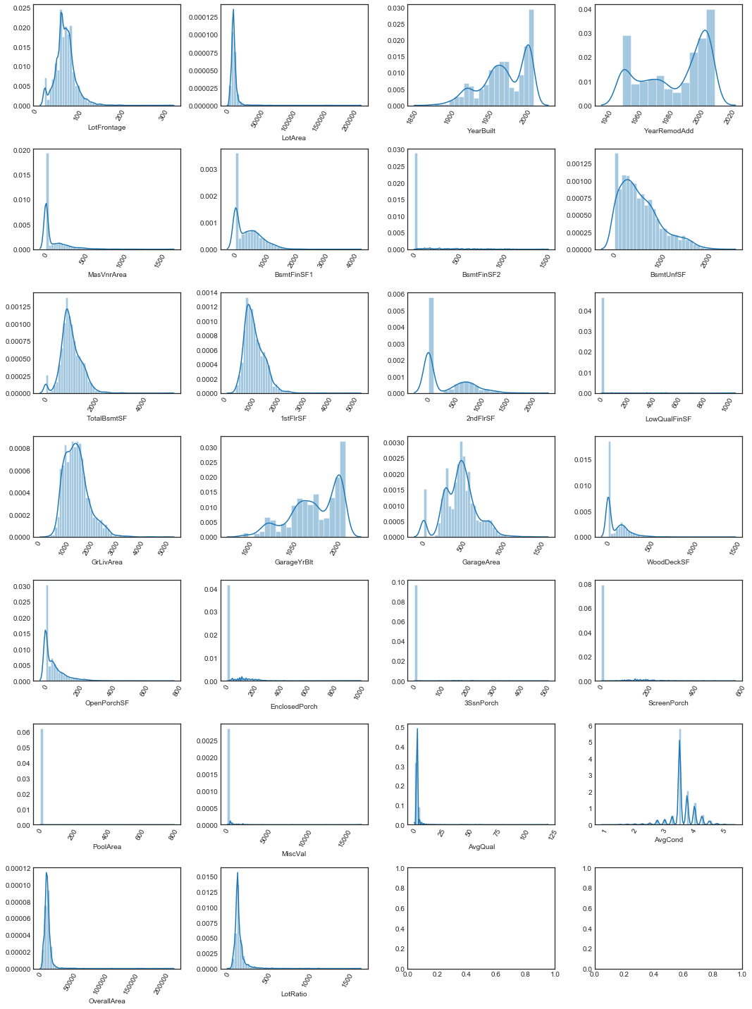
plot_cont_dists(nrows=7, ncols=4, data=quants_data.drop(columns=['SalePrice']), figsize=(15, 20))
# find minimum value over all quantitatives
quants_min_nonzero = quants_data[quants_data != 0].min().min()
print(f"Minimum quantitative value is {quants_data.min().min()}")
print(f"Minimum nonzero quantitative value is {quants_min_nonzero}")
Minimum quantitative value is 0.0
Minimum nonzero quantitative value is 0.4444444444444444
Since the minimum nonzero quantitative value is , we must set (quants_min) if in order not to interfere with monotonicity
# Columns to log transform
log_cols = quants_data.columns.drop(['YearBuilt', 'YearRemodAdd', 'GarageYrBlt', 'GarageArea', 'AvgCond'])
log_cols
Index(['LotFrontage', 'LotArea', 'MasVnrArea', 'BsmtFinSF1', 'BsmtFinSF2',
       'BsmtUnfSF', 'TotalBsmtSF', '1stFlrSF', '2ndFlrSF', 'LowQualFinSF',
       'GrLivArea', 'WoodDeckSF', 'OpenPorchSF', 'EnclosedPorch', '3SsnPorch',
       'ScreenPorch', 'PoolArea', 'MiscVal', 'SalePrice', 'AvgQual',
       'OverallArea', 'LotRatio'],
      dtype='object')
# log transform SalePrice
clean.data = log_transform(data=clean.data, log_cols=['SalePrice'])
drop.data = log_transform(data=drop.data, log_cols=['SalePrice'])
# log transform most quantitatives
clean_edit.data = log_transform(data=clean_edit.data, log_cols=log_cols)
drop_edit.data = log_transform(data=drop_edit.data, log_cols=log_cols)
Model selection and tuning
Create modeling datasets
# set col kinds attribute of HPDataFramePlus attribute for model data method
do_col_kinds(drop)
do_col_kinds(drop_edit)
do_col_kinds(clean)
do_col_kinds(clean_edit)
# model data
mclean = HPDataFramePlus(data=clean.get_model_data(response='log_SalePrice'))
mclean_edit = HPDataFramePlus(data=clean_edit.get_model_data(response='log_SalePrice'))
mdrop = HPDataFramePlus(data=drop.get_model_data(response='log_SalePrice'))
mdrop_edit = HPDataFramePlus(data=drop_edit.get_model_data(response='log_SalePrice'))
mclean.data.info()
<class 'pandas.core.frame.DataFrame'>
MultiIndex: 2916 entries, (train, 1) to (test, 2919)
Columns: 230 entries, LotFrontage to log_SalePrice
dtypes: float64(230)
memory usage: 5.2+ MB
mclean_edit.data.info()
<class 'pandas.core.frame.DataFrame'>
MultiIndex: 2916 entries, (train, 1) to (test, 2919)
Columns: 222 entries, LotShape to log_SalePrice
dtypes: float64(222)
memory usage: 5.0+ MB
mdrop.data.info()
<class 'pandas.core.frame.DataFrame'>
MultiIndex: 2916 entries, (train, 1) to (test, 2919)
Columns: 173 entries, LotFrontage to log_SalePrice
dtypes: float64(173)
memory usage: 4.0+ MB
mdrop_edit.data.info()
<class 'pandas.core.frame.DataFrame'>
MultiIndex: 2916 entries, (train, 1) to (test, 2919)
Columns: 176 entries, LotShape to log_SalePrice
dtypes: float64(176)
memory usage: 4.0+ MB
Compare default models for baseline
hpdfs = [mclean, mdrop, mclean_edit, mdrop_edit]
data_names = ['clean', 'drop', 'clean_edit', 'drop_edit']
response = 'log_SalePrice'
model_data = build_model_data(hpdfs, data_names, response)
First we’ll look at a selection of untuned models with default parameters to get a rough idea of which ones might have better performance.
We’ll use root mean squared error (RMSE) for our loss function. Since we have a relatively small dataset, we’ll use cross-validation to estimate rmse for test data.
# fit some default regressor models
def_models = {'lasso': Lasso(),
              'ridge': Ridge(),
              'bridge': BayesianRidge(),
              'pls': PLSRegression(),
              'svr': SVR(),
              'knn': KNeighborsRegressor(),
              'mlp': MLPRegressor(),
              'dectree': DecisionTreeRegressor(random_state=27),
              'extratree': ExtraTreeRegressor(random_state=27),
              'xgb': XGBRegressor(objective='reg:squarederror', random_state=27, n_jobs=-1)}


fit_def_models = fit_default_models(model_data, def_models)
# compare default models
def_comp_df = compare_performance(fit_def_models, model_data, random_state=27)
def_comp_df.sort_values(by=('clean', 'cv_rmse')).reset_index(drop=True)
| data | model | clean | drop | clean_edit | drop_edit | ||||
|---|---|---|---|---|---|---|---|---|---|
| performance | train_rmse | cv_rmse | train_rmse | cv_rmse | train_rmse | cv_rmse | train_rmse | cv_rmse | |
| 0 | bridge | 0.0950012 | 0.115226 | 0.0988284 | 0.11371 | 0.094478 | 0.11409 | 0.0996576 | 0.115962 |
| 1 | ridge | 0.0948572 | 0.116246 | 0.099311 | 0.114194 | 0.094225 | 0.113706 | 0.0998434 | 0.116375 |
| 2 | xgb | 0.0853461 | 0.122093 | 0.0895599 | 0.123479 | 0.0876669 | 0.123595 | 0.0889219 | 0.126636 |
| 3 | pls | 0.122064 | 0.127405 | 0.127452 | 0.133998 | 0.130416 | 0.13708 | 0.133912 | 0.139404 |
| 4 | svr | 0.122741 | 0.134491 | 0.123251 | 0.13529 | 0.120197 | 0.131894 | 0.123082 | 0.134709 |
| 5 | mlp | 0.116434 | 0.172462 | 0.123199 | 0.182601 | 0.113073 | 0.162779 | 0.122168 | 0.171919 |
| 6 | dectree | 2.93011e-05 | 0.200113 | 2.52372e-05 | 0.205864 | 3.15449e-05 | 0.206949 | 2.48969e-05 | 0.200551 |
| 7 | knn | 0.164677 | 0.20921 | 0.161079 | 0.201135 | 0.153413 | 0.194985 | 0.153466 | 0.18835 |
| 8 | extratree | 2.26808e-05 | 0.211913 | 1.40429e-05 | 0.216413 | 1.66016e-05 | 0.209181 | 1.87349e-05 | 0.213926 |
| 9 | lasso | 0.399557 | 0.399865 | 0.399557 | 0.399721 | 0.399557 | 0.400058 | 0.399557 | 0.399743 |
# compare train and cv performance for each dataset
data_palette = {'train_rmse': 'cornflowerblue', 'cv_rmse': 'midnightblue'}
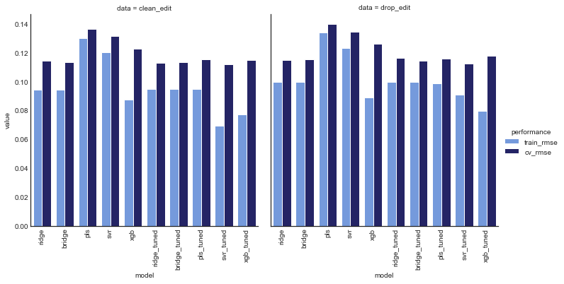
plot_model_comp(def_comp_df, col='data', hue='performance', kind='bar',
palette=data_palette, col_wrap=2)
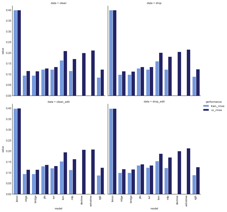
Unsurprisingly, all models (with the exception of lasso regression) had worse CV error than train error. However, for some models the difference was much greater, and these are likely overfitting. In particular, dectree, extratree had cv error roughly 5 orders of magnitude greater than train error, and mlp, knn, and xgb also saw significant increases.
The other models (ridge, bridge, pls and svr) saw slighter differences in cv and train errors, and are thus less likely overfitting.
# compare train and cv error across datasets
perf_palette = {'drop': 'midnightblue', 'clean': 'forestgreen', 'drop_edit': 'crimson',
'clean_edit': 'darkorange'}
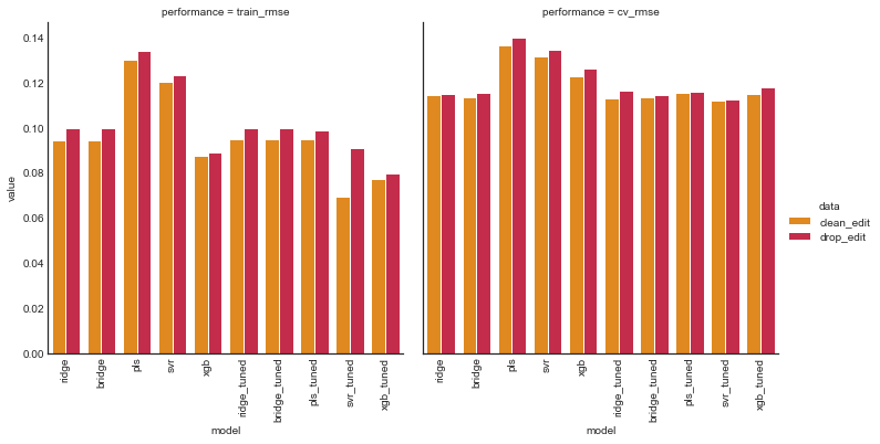
plot_model_comp(def_comp_df, col='performance', hue='data', kind='bar',
palette=perf_palette)
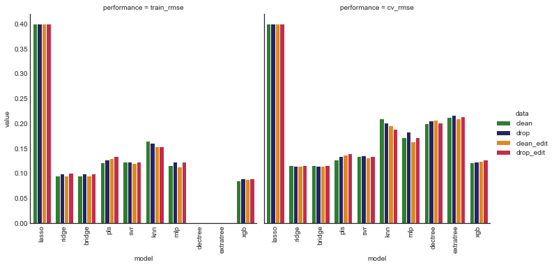
Based on cv rmse, the most promising models appear to be ridge, bridge, xgb, svr, and pls, which are ridge, Bayesian ridge, gradient boosted decision tree, support vector and partial least squared regressors, respectively.
drop_cols = [(data_name, 'train_rmse') for data_name in data_names]
def_comp_cv = def_comp_df.drop(columns=drop_cols).sort_values(by=('clean', 'cv_rmse'))
def_comp_cv
| data | model | clean | drop | clean_edit | drop_edit |
|---|---|---|---|---|---|
| performance | cv_rmse | cv_rmse | cv_rmse | cv_rmse | |
| 2 | bridge | 0.115226 | 0.11371 | 0.11409 | 0.115962 |
| 1 | ridge | 0.116246 | 0.114194 | 0.113706 | 0.116375 |
| 9 | xgb | 0.122093 | 0.123479 | 0.123595 | 0.126636 |
| 3 | pls | 0.127405 | 0.133998 | 0.13708 | 0.139404 |
| 4 | svr | 0.134491 | 0.13529 | 0.131894 | 0.134709 |
| 6 | mlp | 0.172462 | 0.182601 | 0.162779 | 0.171919 |
| 7 | dectree | 0.200113 | 0.205864 | 0.206949 | 0.200551 |
| 5 | knn | 0.20921 | 0.201135 | 0.194985 | 0.18835 |
| 8 | extratree | 0.211913 | 0.216413 | 0.209181 | 0.213926 |
| 0 | lasso | 0.399865 | 0.399721 | 0.400058 | 0.399743 |
Almost all models had an improvement in cv rmse when features were added, so it appears the feature engineering was warranted.
# top models by cv performance for each data set
rank_models_on_data(def_comp_cv, model_data)
| data | model | clean | drop | clean_edit | drop_edit |
|---|---|---|---|---|---|
| performance | cv_rmse | cv_rmse | cv_rmse | cv_rmse | |
| 2 | bridge | 1 | 1 | 2 | 1 |
| 1 | ridge | 2 | 2 | 1 | 2 |
| 9 | xgb | 3 | 3 | 3 | 3 |
| 3 | pls | 4 | 4 | 5 | 5 |
| 4 | svr | 5 | 5 | 4 | 4 |
| 6 | mlp | 6 | 6 | 6 | 6 |
| 7 | dectree | 7 | 8 | 8 | 8 |
| 5 | knn | 8 | 7 | 7 | 7 |
| 8 | extratree | 9 | 9 | 9 | 9 |
| 0 | lasso | 10 | 10 | 10 | 10 |
The top five models were consistent across all four versions of the dataset, and were the promising models identified earlier. In order, they are ridge, bridge, xgb, with svr and pls tied for fourth.
# rank model performance across data sets
rank_models_across_data(def_comp_cv, model_data)
| data | model | clean | drop | clean_edit | drop_edit |
|---|---|---|---|---|---|
| performance | cv_rmse | cv_rmse | cv_rmse | cv_rmse | |
| 2 | bridge | 3 | 1 | 2 | 4 |
| 1 | ridge | 3 | 2 | 1 | 4 |
| 9 | xgb | 1 | 2 | 3 | 4 |
| 3 | pls | 1 | 2 | 3 | 4 |
| 4 | svr | 2 | 4 | 1 | 3 |
| 6 | mlp | 3 | 4 | 1 | 2 |
| 7 | dectree | 1 | 3 | 4 | 2 |
| 5 | knn | 4 | 3 | 2 | 1 |
| 8 | extratree | 2 | 4 | 1 | 3 |
| 0 | lasso | 3 | 1 | 4 | 2 |
The top model, ridge performed best on clean_edit and drop_edit. The next best model, bridge performed best on clean and clean_edit. Third and fourth xgb and pls performed best on clean and drop. Finally svr performed best on clean_edit and drop_edit.
Tune best individual models
Here we’ll focus on tuning the most promising models from the last section. We’ll use both clean_edit and drop_edit since the top model performed best on these.
# retain top 5 models
drop_models = ['lasso', 'dectree', 'extratree', 'knn', 'mlp']
models = remove_models(fit_def_models, drop_models)
try:
    # drop models for clean and drop data
    models.pop('clean')
    models.pop('drop')
    # drop clean and drop data
    model_data.pop('clean')
    model_data.pop('drop')
except KeyError:
    pass

print(f'Promising models are {list(models["clean_edit"].keys())}')
Promising models are ['ridge', 'bridge', 'pls', 'svr', 'xgb']
# train test input output for clean_edit (y_test values are NaN)
X_ce_train = model_data['clean_edit']['X_clean_edit_train']
X_ce_test = model_data['clean_edit']['X_clean_edit_test']
y_ce_train = model_data['clean_edit']['y_clean_edit_train']

# train test input output for clean_edit (y_test values are NaN)
X_de_train = model_data['drop_edit']['X_drop_edit_train']
X_de_test = model_data['drop_edit']['X_drop_edit_test']
y_de_train = model_data['drop_edit']['y_drop_edit_train']
Ridge regression
Ridge regression is linear least squares with an regularization term. We’ll fit default ridge regression models and then tune for comparison.
# Default ridge regression models
ridge_models = defaultdict(dict)
ridge_models['clean_edit']['ridge_def'] = Ridge().fit(X_ce_train, y_ce_train)
ridge_models['drop_edit']['ridge_def'] = Ridge().fit(X_de_train, y_de_train)
Bayesian hyperparameter optimization is an efficient tuning method. We’ll optimize with respect to cv rmse
# ridge regression hyperparameters search space
ridge_space = {'alpha': hp.loguniform('alpha', low=-3*np.log(10), high=2*np.log(10))}

# container for hyperparameter search trials and results
model_ho_results = defaultdict(dict)

# store trial objects for restarting training
model_ho_results['clean_edit']['ridge_tuned'] = {'trials': Trials(), 'params': None}
model_ho_results['drop_edit']['ridge_tuned'] = {'trials': Trials(), 'params': None}
# optimize hyperparameters
model_ho_results['clean_edit']['ridge_tuned'] = \
                ho_results(obj=ho_cv_rmse, space=ridge_space,
                           est_name='ridge', X_train=X_ce_train,
                           y_train=y_ce_train,
                           max_evals=100, random_state=27,
                           trials=model_ho_results['clean_edit']['ridge_tuned']['trials'])
model_ho_results['drop_edit']['ridge_tuned'] = \
                ho_results(obj=ho_cv_rmse, space=ridge_space,
                           est_name='ridge', X_train=X_de_train,
                           y_train=y_de_train,
                           max_evals=100, random_state=27,
                           trials=model_ho_results['drop_edit']['ridge_tuned']['trials'])
100%|██████████| 100/100 [00:08<00:00, 11.38it/s, best loss: 0.11253072830975036]
100%|██████████| 100/100 [00:07<00:00, 13.32it/s, best loss: 0.11564439386901282]
%%capture
# create and fit models with optimal hyperparameters
ridge_models['clean_edit']['ridge_tuned'] = \
                    Ridge(**model_ho_results['clean_edit']['ridge_tuned']['params'])
ridge_models['drop_edit']['ridge_tuned'] = \
                    Ridge(**model_ho_results['drop_edit']['ridge_tuned']['params'])
ridge_models['clean_edit']['ridge_tuned'].fit(X_ce_train, y_ce_train)
ridge_models['drop_edit']['ridge_tuned'].fit(X_de_train, y_de_train)
# compare Ridge regression models
compare_performance(ridge_models, model_data, random_state=27)
| data | model | clean_edit | drop_edit | ||
|---|---|---|---|---|---|
| performance | train_rmse | cv_rmse | train_rmse | cv_rmse | |
| 0 | ridge_def | 0.094225 | 0.11256 | 0.0998434 | 0.115635 |
| 1 | ridge_tuned | 0.0950445 | 0.11315 | 0.0996629 | 0.114869 |
The ridge regression model trained on the clean_edit dataset and tuned with Bayesian search had the best cv rmse. We note however that the model trained on drop_edit had a , which is promising (a lower train rmse might indicate overfitting).
Since ridge regression is just linear regression with a regularization term, it’s relatively straightfoward to interpret. We’ll rank the features of the best model their coefficient weights.
# Top and bottom 10 features in best ridge model
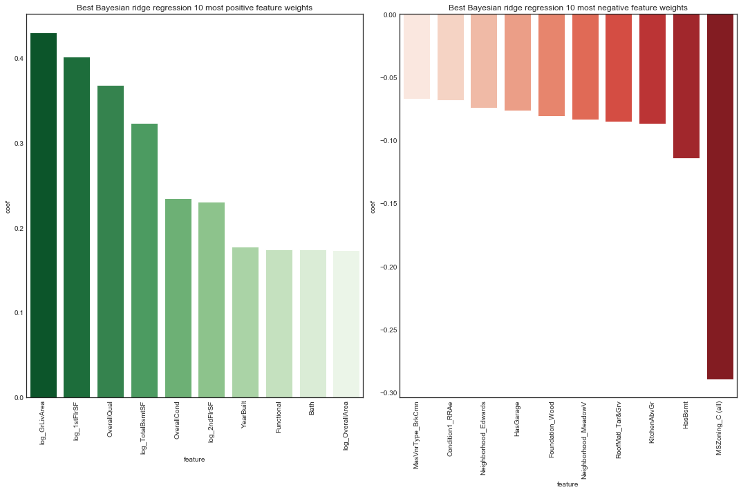
plot_features(ridge_models['clean_edit']['ridge_tuned'], 'ridge regression', X_ce_train, 10,
figsize=(15, 10), rotation=90)
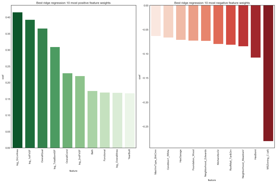
The rankings of most positive feature weights are not too suprising. The most postively weighted feature was overall quality. We note condition variables and size variables are prominent.
The rankings of most negative feature weights are perhaps more surprising, in particular the presence of a basement and number of kitchens. Interestingly, several neighborhoods stand out as having a negative association with sale price. The most negatively weighted feature was the property being zoned commercial.
# add tuned ridge models
models['clean_edit']['ridge_tuned'] = ridge_models['clean_edit']['ridge_tuned']
models['drop_edit']['ridge_tuned'] = ridge_models['drop_edit']['ridge_tuned']
Bayesian Ridge regression
Bayesian ridge regression is similar to ridge regression except it uses Bayesian methods to estimate the regularization parameter from the data.
# Default Bayesian Ridge models
bridge_models = defaultdict(dict)
bridge_models['clean_edit']['bridge_def'] = BayesianRidge().fit(X_ce_train, y_ce_train)
bridge_models['drop_edit']['bridge_def'] = BayesianRidge().fit(X_de_train, y_de_train)
# bayesian ridge regression hyperparameter space
bridge_space = {'alpha_1': hp.loguniform('alpha_1', low=-9*np.log(10), high=3*np.log(10)),
                'alpha_2': hp.loguniform('alpha_2', low=-9*np.log(10), high=3*np.log(10)),
                'lambda_1': hp.loguniform('lambda_1', low=-9*np.log(10), high=3*np.log(10)),
                'lambda_2': hp.loguniform('lambda_2', low=-9*np.log(10), high=3*np.log(10))}

# store trial objects for restarting training
model_ho_results['clean_edit']['bridge_tuned'] = {'trials': Trials(), 'params': None}
model_ho_results['drop_edit']['bridge_tuned'] = {'trials': Trials(), 'params': None}
# optimize hyperparameters
model_ho_results['clean_edit']['bridge_tuned'] = \
                ho_results(obj=ho_cv_rmse, space=bridge_space,
                           est_name='bridge', X_train=X_ce_train,
                           y_train=y_ce_train,
                           max_evals=100, random_state=27,
                           trials=model_ho_results['clean_edit']['bridge_tuned']['trials'])
model_ho_results['drop_edit']['bridge_tuned'] = \
                ho_results(obj=ho_cv_rmse, space=bridge_space,
                           est_name='bridge', X_train=X_de_train,
                           y_train=y_de_train,
                           max_evals=100, random_state=27,
                           trials=model_ho_results['drop_edit']['bridge_tuned']['trials'])
100%|██████████| 100/100 [00:37<00:00,  2.67it/s, best loss: 0.11254203419476108]
100%|██████████| 100/100 [00:27<00:00,  3.66it/s, best loss: 0.11576647439940951]
%%capture
# add and fit models with optimal hyperparameters
bridge_models['clean_edit']['bridge_tuned'] = \
            BayesianRidge(**model_ho_results['clean_edit']['bridge_tuned']['params'])
bridge_models['drop_edit']['bridge_tuned'] = \
            BayesianRidge(**model_ho_results['drop_edit']['bridge_tuned']['params'])
bridge_models['clean_edit']['bridge_tuned'].fit(X_ce_train, y_ce_train)
bridge_models['drop_edit']['bridge_tuned'].fit(X_de_train, y_de_train)
# compare Ridge regression models
compare_performance(bridge_models, model_data, random_state=27)
| data | model | clean_edit | drop_edit | ||
|---|---|---|---|---|---|
| performance | train_rmse | cv_rmse | train_rmse | cv_rmse | |
| 0 | bridge_def | 0.094478 | 0.113612 | 0.0996576 | 0.114887 |
| 1 | bridge_tuned | 0.09467 | 0.114397 | 0.0996135 | 0.115072 |
As with ordinary ridge regression, the Bayesian ridge model trained on the clean_edit data and tuned with Bayesian search had the best cv rmse.
As with ridge regression, the model is straightforward to interpret.
# Top and bottom 10 features in best Bayesian ridge model
plot_features(bridge_models['clean_edit']['bridge_tuned'], 'Bayesian ridge regression', X_ce_train, 10,
             figsize=(15, 10), rotation=90)
Feature weight rankings are nearly identical to the ridge model.
# add tuned bridge models
models['clean_edit']['bridge_tuned'] = bridge_models['clean_edit']['bridge_tuned']
models['drop_edit']['bridge_tuned'] = bridge_models['drop_edit']['bridge_tuned']
Partial Least Squares
Partial least squares regression stands out among the other models we’re tuning here as the only dimensional reduction method. It is well-suited to multicollinearity in the input data.
# Default partial least squares models
pls_models = defaultdict(dict)
pls_models['clean_edit']['pls_def'] = PLSRegression().fit(X_ce_train, y_ce_train)
pls_models['drop_edit']['pls_def'] = PLSRegression().fit(X_de_train, y_de_train)
The main hyperparameter of interest in partial least squared is the number of components (analogous to the number of components in principal component analysis) which is essentially the number of dimensions of the reduced dataset.
# partial least squares hyperparameter spaces
pls_ce_space = {'max_iter': ho_scope.int(hp.quniform('max_iter', low=200,
                                                     high=10000, q=10)),
               'n_components': ho_scope.int(hp.quniform('n_components', low=2,
                                                        high=X_ce_train.shape[1] - 2, q=1))
                }
pls_de_space = {'max_iter': ho_scope.int(hp.quniform('max_iter', low=200,
                                                     high=10000, q=10)),
               'n_components': ho_scope.int(hp.quniform('n_components', low=2,
                                                        high=X_de_train.shape[1] - 2, q=1))}

# store trial objects for restarting training
model_ho_results['clean_edit']['pls_tuned'] = {'trials': Trials(), 'params': None}
model_ho_results['drop_edit']['pls_tuned'] = {'trials': Trials(), 'params': None}
# optimize hyperparameters
model_ho_results['clean_edit']['pls_tuned'] = \
                ho_results(obj=ho_cv_rmse, space=pls_ce_space, est_name='pls',
                           X_train=X_ce_train, y_train=y_ce_train, max_evals=100,
                           random_state=27,
                           trials=model_ho_results['clean_edit']['pls_tuned']['trials'])
model_ho_results['drop_edit']['pls_tuned'] = \
                ho_results(obj=ho_cv_rmse, space=pls_de_space, est_name='pls',
                           X_train=X_de_train, y_train=y_de_train, max_evals=100,
                           random_state=27,
                           trials=model_ho_results['drop_edit']['pls_tuned']['trials'])
100%|██████████| 100/100 [01:30<00:00,  1.11it/s, best loss: 0.11628329440486904]
100%|██████████| 100/100 [01:02<00:00,  1.60it/s, best loss: 0.11672287624670073]
%%capture
# workaround to cast results of hyperopt param search to correct type
conv_params = ['max_iter', 'n_components']
model_ho_results['clean_edit']['pls_tuned']['params'] = \
            convert_to_int(model_ho_results['clean_edit']['pls_tuned']['params'],
                           conv_params)
model_ho_results['drop_edit']['pls_tuned']['params'] = \
            convert_to_int(model_ho_results['drop_edit']['pls_tuned']['params'],
                           conv_params)

# add and fit models with optimal hyperparameters
pls_models['clean_edit']['pls_tuned'] = \
            PLSRegression(**model_ho_results['clean_edit']['pls_tuned']['params'])
pls_models['drop_edit']['pls_tuned'] = \
            PLSRegression(**model_ho_results['drop_edit']['pls_tuned']['params'])
pls_models['clean_edit']['pls_tuned'].fit(X_ce_train, y_ce_train)
pls_models['drop_edit']['pls_tuned'].fit(X_de_train, y_de_train)
# inspect pls optimal parameters
print(f"On the clean_edit data, optimal PLS parameters are: \n\t {model_ho_results['clean_edit']['pls_tuned']['params']}")
print(f"On the drop_edit data, optimal PLS parameters are: \n\t {model_ho_results['drop_edit']['pls_tuned']['params']}")
On the clean_edit data, optimal PLS parameters are:
	 {'max_iter': 5690, 'n_components': 12}
On the drop_edit data, optimal PLS parameters are:
	 {'max_iter': 2640, 'n_components': 16}
Interestingly, only a small number of components were deemed optimal! It’s worth recalling that this likely reflects a local minimum in the loss function, so the result should be taken with a grain of salt. However, it is interesting to note that such a low number of components are sufficient to get a competitive model.
# compare Bayesian Ridge models on clean and edit datasets
compare_performance(pls_models, model_data)
| data | model | clean_edit | drop_edit | ||
|---|---|---|---|---|---|
| performance | train_rmse | cv_rmse | train_rmse | cv_rmse | |
| 0 | pls_def | 0.130416 | 0.136774 | 0.133912 | 0.139224 |
| 1 | pls_tuned | 0.0948243 | 0.115228 | 0.0989862 | 0.116016 |
In contrast to ridge and Bayesian ridge regression, the tuned partial least squares had slightly lower cv rmse on the drop_edit dataset. This cv rmse is very close to that of tuned ridge and Bayesian ridge models – it’s remarkable that only 16 components are required!
# add tuned pls models
models['clean_edit']['pls_tuned'] = pls_models['clean_edit']['pls_tuned']
models['drop_edit']['pls_tuned'] = pls_models['drop_edit']['pls_tuned']
Support Vector Machine
# Default support vector models
svr_models = defaultdict(dict)
svr_models['clean_edit']['svr_def'] = SVR().fit(X_ce_train, y_ce_train)
svr_models['drop_edit']['svr_def'] = SVR().fit(X_de_train, y_de_train)
# hyperparameter space for SVR with rbf kernel
svr_space = {'gamma': hp.loguniform('gamma', low=-3*np.log(10), high=2*np.log(10)),
             'C': hp.loguniform('C', low=-3*np.log(10), high=2*np.log(10)),
             'epsilon': hp.loguniform('epsilon', low=-3*np.log(10), high=2*np.log(10))
            }

# store trial objects for restarting training
model_ho_results['clean_edit']['svr_tuned'] = {'trials': Trials(), 'params': None}
model_ho_results['drop_edit']['svr_tuned'] = {'trials': Trials(), 'params': None}
# optimize hyperparameters
model_ho_results['clean_edit']['svr_tuned'] = \
            ho_results(obj=ho_cv_rmse, space=svr_space, est_name='svr',
                       X_train=X_ce_train, y_train=y_ce_train, max_evals=50,
                       random_state=27,
                       trials=model_ho_results['clean_edit']['svr_tuned']['trials'])
model_ho_results['drop_edit']['svr_tuned'] = \
            ho_results(obj=ho_cv_rmse, space=svr_space, est_name='svr',
                       X_train=X_de_train, y_train=y_de_train, max_evals=50,
                       random_state=27,
                       trials=model_ho_results['drop_edit']['svr_tuned']['trials'])
100%|██████████| 50/50 [01:37<00:00,  1.95s/it, best loss: 0.11318101455546818]
100%|██████████| 50/50 [01:32<00:00,  1.84s/it, best loss: 0.11424890264814005]
%%capture
# fit models with optimal hyperparameters
svr_models['clean_edit']['svr_tuned'] = \
                        SVR(**model_ho_results['clean_edit']['svr_tuned']['params'])
svr_models['drop_edit']['svr_tuned'] = \
                        SVR(**model_ho_results['drop_edit']['svr_tuned']['params'])
svr_models['clean_edit']['svr_tuned'].fit(X_ce_train, y_ce_train)
svr_models['drop_edit']['svr_tuned'].fit(X_de_train, y_de_train)
# compare SVR model performance on clean and edit datasets
svr_comp_df = compare_performance(svr_models, model_data)
svr_comp_df
As with all previous models, we’re seeing better performance on drop_edit. Again, a higher train rmse on drop_edit but a lower cv rmse is a positive sign.
# add tuned svr models
models['clean_edit']['svr_tuned'] = svr_models['clean_edit']['svr_tuned']
models['drop_edit']['svr_tuned'] = svr_models['drop_edit']['svr_tuned']
Gradient boosted trees
# Default gradient boost tree models
xgb_models = defaultdict(dict)
xgb_models['clean_edit']['xgb_def'] = XGBRegressor(objective='reg:squarederror', random_state=27, n_jobs=-1)
xgb_models['drop_edit']['xgb_def'] = XGBRegressor(objective='reg:squarederror', random_state=27, n_jobs=-1)
xgb_models['clean_edit']['xgb_def'].fit(X_ce_train.values, y_ce_train.values)
xgb_models['drop_edit']['xgb_def'].fit(X_de_train.values, y_de_train.values)
XGBRegressor(base_score=0.5, booster='gbtree', colsample_bylevel=1,
             colsample_bynode=1, colsample_bytree=1, gamma=0,
             importance_type='gain', learning_rate=0.1, max_delta_step=0,
             max_depth=3, min_child_weight=1, missing=None, n_estimators=100,
             n_jobs=-1, nthread=None, objective='reg:squarederror',
             random_state=27, reg_alpha=0, reg_lambda=1, scale_pos_weight=1,
             seed=None, silent=None, subsample=1, verbosity=1)
# hyperparameter spaces
xgb_space = {'max_depth': ho_scope.int(hp.quniform('max_depth', low=1, high=3, q=1)),
             'n_estimators': ho_scope.int(hp.quniform('n_estimators', low=100, high=500, q=50)),
             'learning_rate': hp.loguniform('learning_rate', low=-4*np.log(10), high=0),
             'gamma': hp.loguniform('gamma', low=-3*np.log(10), high=2*np.log(10)),
             'min_child_weight': ho_scope.int(hp.quniform('min_child_weight', low=1, high=7, q=1)),
             'subsample': hp.uniform('subsample', low=0.25, high=1),
             'colsample_bytree': hp.uniform('colsample_bytree', low=0.25, high=1),
             'colsample_bylevel': hp.uniform('colsample_bylevel', low=0.25, high=1),
             'colsample_bynode': hp.uniform('colsample_bynode', low=0.25, high=1),
             'reg_lambda': hp.loguniform('reg_lambda', low=-2*np.log(10), high=2*np.log(10)),
             'reg_alpha': hp.loguniform('reg_alpha', low=-1*np.log(10), high=1*np.log(10)),
            }

# store trial objects for restarting training
model_ho_results['clean_edit']['xgb_tuned'] = {'trials': Trials(), 'params': None}
model_ho_results['drop_edit']['xgb_tuned'] = {'trials': Trials(), 'params': None}
# optimize hyperparameters
model_ho_results['clean_edit']['xgb_tuned'] = \
            ho_results(obj=ho_cv_rmse, space=xgb_space, est_name='xgb',
                       X_train=X_ce_train, y_train=y_ce_train, max_evals=50,
                       random_state=27,
                       trials=model_ho_results['clean_edit']['xgb_tuned']['trials'])
model_ho_results['drop_edit']['xgb_tuned'] = \
            ho_results(obj=ho_cv_rmse, space=xgb_space, est_name='xgb',
                       X_train=X_de_train, y_train=y_de_train, max_evals=50,
                       random_state=27,
                       trials=model_ho_results['drop_edit']['xgb_tuned']['trials'])
100%|██████████| 50/50 [09:51<00:00, 11.82s/it, best loss: 0.11487854997487522]
100%|██████████| 50/50 [08:56<00:00, 10.74s/it, best loss: 0.12018590987034897]
%%capture
# convert params to int
conv_params = ['max_depth', 'min_child_weight', 'n_estimators']
model_ho_results['clean_edit']['xgb_tuned']['params'] = \
        convert_to_int(model_ho_results['clean_edit']['xgb_tuned']['params'], conv_params)
model_ho_results['clean_edit']['xgb_tuned']['params'] = \
        convert_to_int(model_ho_results['clean_edit']['xgb_tuned']['params'], conv_params)

# add and fit models with optimal hyperparameters
fixed_params = {'objective': 'reg:squarederror', 'n_jobs': -1, 'random_state': 27}
xgb_models['clean_edit']['xgb_tuned'] = \
        XGBRegressor(**{**model_ho_results['clean_edit']['xgb_tuned']['params'],
                        **fixed_params})
xgb_models['drop_edit']['xgb_tuned'] = \
        XGBRegressor(**{**model_ho_results['clean_edit']['xgb_tuned']['params'],
                        **fixed_params})
xgb_models['clean_edit']['xgb_tuned'].fit(X_ce_train.values, y_ce_train.values)
xgb_models['drop_edit']['xgb_tuned'].fit(X_de_train.values, y_de_train.values)
# compare XGBoost models on clean_edit and drop_edit datasets
xgb_comp_df = compare_performance(xgb_models, model_data)
xgb_comp_df
| data | model | clean_edit | drop_edit | ||
|---|---|---|---|---|---|
| performance | train_rmse | cv_rmse | train_rmse | cv_rmse | |
| 0 | xgb_def | 0.0876669 | 0.125045 | 0.0889219 | 0.125903 |
| 1 | xgb_tuned | 0.0772716 | 0.113871 | 0.0795258 | 0.117488 |
In contrast to all previous models, the gradient boosted tree regressor had a lower cv rmse on clean_edit, but similarly to previous models train rmse was higher.
We can rank the features by importance (in this case, the number of times the feature was used to split a tree across all trees in the forest).
# top 20 feature importances of xgb model on drop_edit data
plot_xgb_features(xgb_models['drop_edit']['xgb_tuned'], X_de_train, 10, figsize=(10, 8),
                  rotation=90)
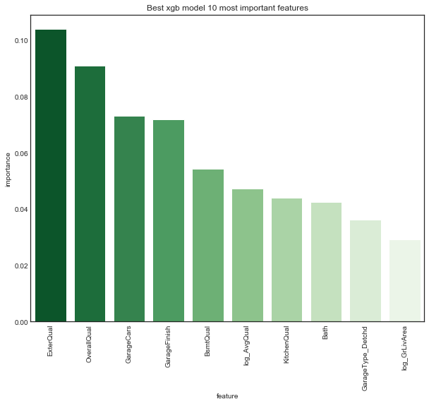
On the drop_edit data, the top ten features for the gradient boosted trees regression model seem quite different from the top ten features of ridge regression. Only OverallQual and log_GrLivArea appear in both, and whereas both rank OverallQual third, ridge ranks log_GrLivArea first while xgb ranks it tenth. While the top ridge features seemed plausible and natural, some of the top xgb features seem more surpising, especially the highest ranked feature GarageType_Detached.
# replace default models with tuned models
models['clean_edit']['xgb_tuned'] = xgb_models['clean_edit']['xgb_tuned']
models['drop_edit']['xgb_tuned'] = xgb_models['drop_edit']['xgb_tuned']
Compare tuned models and save parameters
# compare results of tuned models
tuned_comp_df = compare_performance(models, model_data, random_state=27)
tuned_comp_df.sort_values(by=('clean_edit', 'cv_rmse')).reset_index(drop=True)
| data | model | clean_edit | drop_edit | ||
|---|---|---|---|---|---|
| performance | train_rmse | cv_rmse | train_rmse | cv_rmse | |
| 0 | svr_tuned | 0.06929 | 0.112236 | 0.0911838 | 0.112445 |
| 1 | ridge_tuned | 0.0950445 | 0.113011 | 0.0996629 | 0.116393 |
| 2 | bridge_tuned | 0.09467 | 0.113658 | 0.0996135 | 0.114628 |
| 3 | bridge | 0.094478 | 0.113733 | 0.0996576 | 0.115385 |
| 4 | ridge | 0.094225 | 0.114597 | 0.0998434 | 0.11497 |
| 5 | xgb_tuned | 0.0772716 | 0.114933 | 0.0795258 | 0.11772 |
| 6 | pls_tuned | 0.0948243 | 0.115411 | 0.0989862 | 0.115752 |
| 7 | xgb | 0.0876669 | 0.123048 | 0.0889219 | 0.126444 |
| 8 | svr | 0.120197 | 0.131465 | 0.123082 | 0.134494 |
| 9 | pls | 0.130416 | 0.136702 | 0.133912 | 0.140016 |
# compare tuned model train and cv performance on clean and edit datasets
plot_model_comp(tuned_comp_df, col='data', hue='performance', kind='bar', palette=data_palette)
# compare clean and edit performance for train and cv error
plot_model_comp(tuned_comp_df, col='performance', hue='data', kind='bar', palette=perf_palette)
# pickle hyperopt trials and results
pickle_to_file(model_ho_results, '../training/model_tuning_results.pkl')

# pickle tuned models
pickle_to_file(models, '../training/tuned_models.pkl')
Ensembles
# unpickle tuned models from last section
tuned_models = pickle_from_file('../training/tuned_models.pkl')
Voting
Voting ensembles predict a weighted average of base models.
We’ll use the implementation sklearn.ensemble.VotingRegressor. Unfortunately sklearn.PLSRegressor’s predict method returns arrays of size (n_samples, 1) rather than (n_samples,) like all all other models. This throws an error when passed in as an estimator to cross_val_score so we won’t use it as a base model. We also won’t use bridge since its feature weights were nearly identical to ridge, so in the end our voting regressor will consist of three base models: ridge, support vector and gradient boosted tree regression.
tuned_models['clean_edit'].keys()
dict_keys(['ridge', 'bridge', 'pls', 'svr', 'xgb', 'ridge_tuned', 'bridge_tuned', 'pls_tuned', 'svr_tuned', 'xgb_tuned'])
drop_models = ['ridge', 'bridge', 'pls', 'svr', 'xgb', 'bridge_tuned',
               'pls_tuned']
base_pretuned = remove_models(tuned_models, drop_models)
Default base and uniform weights
For a baseline, we’ll look at a voting ensemble of default base models with uniform weights
%%capture
# Default models for Voting Regressor
base_def = [('ridge', Ridge()),
            ('svr', SVR()),
            ('xgb', XGBRegressor(objective='reg:squarederror', n_jobs=-1, random_state=27))]

# Voting ensembles with uniform weights and untuned base models
ensembles = defaultdict(dict)
ensembles['clean_edit']['voter_def'] = VotingRegressor(base_def, n_jobs=-1)
ensembles['drop_edit']['voter_def'] = VotingRegressor(base_def, n_jobs=-1)
ensembles['clean_edit']['voter_def'].fit(X_ce_train.values, y_ce_train.values)
ensembles['drop_edit']['voter_def'].fit(X_de_train.values, y_de_train.values)
Pretuned base and uniform weights
We also consider a voting ensemble with pretuned base models and uniform weights.
%%capture
# Voting ensmebles with uniform weights for pretuned base models
ensembles['clean_edit']['voter_uniform_pretuned'] = \
         VotingRegressor(list(base_pretuned['clean_edit'].items()), n_jobs=-1)
ensembles['drop_edit']['voter_uniform_pretuned'] = \
         VotingRegressor(list(base_pretuned['drop_edit'].items()), n_jobs=-1)
ensembles['clean_edit']['voter_uniform_pretuned'].fit(X_ce_train.values, y_ce_train.values)
ensembles['drop_edit']['voter_uniform_pretuned'].fit(X_de_train.values, y_de_train.values)
# voting ensemble hyperparameters for pretuned base
weight_space = {'voter1': hp.uniform('voter1', low=0, high=1),
               'voter2': hp.uniform('voter2', low=0, high=1),
               'voter3': hp.uniform('voter3', low=0, high=1)
              }

voter_fixed_params = {'n_jobs': -1}


# container for hyperparameter search trials and results
ens_ho_results = defaultdict(dict)

# store trial objects for restarting training
ens_ho_results['clean_edit']['voter_pretuned'] = {'trials': Trials(), 'params': None}
ens_ho_results['drop_edit']['voter_pretuned'] = {'trials': Trials(), 'params': None}
# optimize weights for voting ensemble with pretuned base
ens_ho_results['clean_edit']['voter_pretuned'] = \
        ho_ens_results(obj=ho_ens_cv_rmse, space=weight_space, ens_name='voter',
                       base_ests=base_pretuned['clean_edit'],
                       X_train=X_ce_train, y_train=y_ce_train,
                       fixed_params=voter_fixed_params,
                       pretuned=True, random_state=27, max_evals=50,
                       trials=ens_ho_results['clean_edit']['voter_pretuned']['trials'])
ens_ho_results['drop_edit']['voter_pretuned'] = \
        ho_ens_results(obj=ho_ens_cv_rmse, space=weight_space, ens_name='voter',
                       base_ests=base_pretuned['drop_edit'],
                       X_train=X_de_train, y_train=y_de_train,
                       fixed_params=voter_fixed_params,
                       pretuned=True, random_state=27, max_evals=50,
                       trials=ens_ho_results['drop_edit']['voter_pretuned']['trials'])
100%|██████████| 50/50 [16:35<00:00, 19.91s/it, best loss: 0.10821736452332247]
100%|██████████| 50/50 [12:22<00:00, 14.85s/it, best loss: 0.11169063598085288]
%%capture
# store and normalize weights
ce_pretuned_weights = list(ens_ho_results['clean_edit']['voter_pretuned']['params'].values())
de_pretuned_weights = list(ens_ho_results['drop_edit']['voter_pretuned']['params'].values())
ce_pretuned_weights = convert_and_normalize_weights(ce_pretuned_weights)
de_pretuned_weights = convert_and_normalize_weights(de_pretuned_weights)

# add and fit voting ensembles of pretuned base estimators with tuned weights
ensembles['clean_edit']['voter_pretuned'] = \
                    VotingRegressor(list(base_pretuned['clean_edit'].items()),
                                    weights=ce_pretuned_weights)
ensembles['drop_edit']['voter_pretuned'] = \
                    VotingRegressor(list(base_pretuned['drop_edit'].items()),
                                    weights=de_pretuned_weights)
ensembles['clean_edit']['voter_pretuned'].fit(X_ce_train.values, y_ce_train.values)
ensembles['drop_edit']['voter_pretuned'].fit(X_de_train.values, y_de_train.values)
Fully tuned voter
Finally, we’ll tune a voting regressors base model hyperparameters and voting weights simultaneously with Bayesian search.
# base hyperparameter spaces
ridge_base_space = {'alpha_ridge': hp.loguniform('alpha_ridge', low=-3*np.log(10), high=2*np.log(10))}
svr_base_space = {'gamma_svr': hp.loguniform('gamma_svr', low=-3*np.log(10), high=2*np.log(10)),
                  'C_svr': hp.loguniform('C_svr', low=-3*np.log(10), high=2*np.log(10)),
                  'epsilon_svr': hp.loguniform('epsilon_svr', low=-3*np.log(10), high=2*np.log(10))}
xgb_base_space = {'max_depth_xgb': ho_scope.int(hp.quniform('max_depth_xgb', low=1, high=3, q=1)),
                  'n_estimators_xgb': ho_scope.int(hp.quniform('n_estimators_xgb', low=100, high=500, q=50)),
                  'learning_rate_xgb': hp.loguniform('learning_rate_xgb', low=-4*np.log(10), high=0),
                  'gamma_xgb': hp.loguniform('gamma_xgb', low=-3*np.log(10), high=2*np.log(10)),
                  'min_child_weight_xgb': ho_scope.int(hp.quniform('min_child_weight_xgb', low=1, high=7, q=1)),
                  'subsample_xgb': hp.uniform('subsample_xgb', low=0.25, high=1),
                  'colsample_bytree_xgb': hp.uniform('colsample_bytree_xgb', low=0.25, high=1),
                  'colsample_bylevel_xgb': hp.uniform('colsample_bylevel_xgb', low=0.25, high=1),
                  'colsample_bynode_xgb': hp.uniform('colsample_bynode_xgb', low=0.25, high=1),
                  'reg_lambda_xgb': hp.loguniform('reg_lambda_xgb', low=-2*np.log(10), high=2*np.log(10)),
                  'reg_alpha_xgb': hp.loguniform('reg_alpha_xgb', low=-1*np.log(10), high=1*np.log(10)),
                 }

# voting ensemble hyperparameters for untuned base
base_space = {**ridge_base_space, **svr_base_space, **xgb_base_space}
voter_space = {**base_space, **weight_space}

# store trial objects for restarting training
ens_ho_results['clean_edit']['voter_tuned'] = {'trials': Trials(), 'params': None}
ens_ho_results['drop_edit']['voter_tuned'] = {'trials': Trials(), 'params': None}
# optimize all voting ensemble hyperparameters jointly
ens_ho_results['clean_edit']['voter_tuned'] = \
            ho_ens_results(obj=ho_ens_cv_rmse, space=voter_space, ens_name='voter',
                           X_train=X_ce_train, y_train=y_ce_train,
                           fixed_params=voter_fixed_params,
                           pretuned=False, random_state=27, max_evals=50,
                           trials=ens_ho_results['clean_edit']['voter_tuned']['trials'])
ens_ho_results['drop_edit']['voter_tuned'] = \
            ho_ens_results(obj=ho_ens_cv_rmse, space=voter_space, ens_name='voter',
                           X_train=X_de_train, y_train=y_de_train,
                           fixed_params=voter_fixed_params,
                           pretuned=False, random_state=27, max_evals=50,
                           trials=ens_ho_results['drop_edit']['voter_tuned']['trials'])
100%|██████████| 50/50 [09:15<00:00, 11.11s/it, best loss: 0.11562031262896297]
100%|██████████| 50/50 [07:55<00:00,  9.51s/it, best loss: 0.11927675656382479]
%%capture
# add and fit fully tuned voting ensembles
ensembles['clean_edit']['voter_tuned'] = \
            voter_from_search_params(ens_ho_results['clean_edit']['voter_tuned']['params'],
                                     X_ce_train, y_ce_train, random_state=27)
ensembles['drop_edit']['voter_tuned'] = \
            voter_from_search_params(ens_ho_results['drop_edit']['voter_tuned']['params'],
                                     X_de_train, y_de_train, random_state=27)
Stacking
Stacking ensembles fit a meta models to the predictions of base models. To avoid overfitting, one can use folds to generate base models predictions.
We’ll use the implementation mlxtend.StackingCVRegressor. We’ll also choose our meta models from the set of base models (ridge, support vector, and gradient boosted tree regression).
Default base and meta
For a baseline, we’ll consider stack ensembles for which both base and meta models have default parameters. We’ll use all three base models for each, and vary the meta model across the base models.
# add default base and meta without using features in secondary
ensembles = add_stacks(ensembles, model_data, suffix='def',
                       use_features_in_secondary=False, random_state=27)
# add default base and meta using features in secondary
ensembles = add_stacks(ensembles, model_data, suffix='def',
                       use_features_in_secondary=True, random_state=27)
Pretuned base and meta
Now we’ll consider stack ensembles for which the base and meta models are already tuned. Again, we’ll use all three base models and vary the meta model across the base models.
# add pretuned base and meta without using features in secondary
ensembles = add_stacks(ensembles, model_data, base_ests=base_pretuned,
                       meta_ests=base_pretuned, suffix='pretuned',
                       use_features_in_secondary=False, random_state=27)
# add pretuned base and meta using features in secondary
ensembles = add_stacks(ensembles, model_data, base_ests=base_pretuned,
                       meta_ests=base_pretuned, suffix='pretuned',
                       use_features_in_secondary=True, random_state=27)
Fully tuned stacks
Finally, we’ll tune stack ensembles at once, that is we’ll tune both base and meta models simultaneously. As before, we’ll use all three base models and vary the meta model across the base models.
# meta hyperparameter spaces
ridge_meta_space = {'alpha_ridge_meta': hp.loguniform('alpha_ridge_meta', low=-3*np.log(10), high=2*np.log(10))}
svr_meta_space = {'gamma_svr_meta': hp.loguniform('gamma_svr_meta', low=-3*np.log(10), high=2*np.log(10)),
                  'C_svr_meta': hp.loguniform('C_svr_meta', low=-3*np.log(10), high=2*np.log(10)),
                  'epsilon_svr_meta': hp.loguniform('epsilon_svr_meta', low=-3*np.log(10), high=2*np.log(10))}
xgb_meta_space = {'max_depth_xgb_meta': ho_scope.int(hp.quniform('max_depth_xgb_meta', low=1, high=3, q=1)),
                  'n_estimators_xgb_meta': ho_scope.int(hp.quniform('n_estimators_xgb_meta', low=100, high=500, q=50)),
                  'learning_rate_xgb_meta': hp.loguniform('learning_rate_xgb_meta', low=-4*np.log(10), high=0),
                  'gamma_xgb_meta': hp.loguniform('gamma_xgb_meta', low=-3*np.log(10), high=2*np.log(10)),
                  'min_child_weight_xgb_meta': ho_scope.int(hp.quniform('min_child_weight_xgb_meta', low=1, high=7, q=1)),
                  'subsample_xgb_meta': hp.uniform('subsample_xgb_meta', low=0.25, high=1),
                  'colsample_bytree_xgb_meta': hp.uniform('colsample_bytree_xgb_meta', low=0.25, high=1),
                  'colsample_bylevel_xgb_meta': hp.uniform('colsample_bylevel_xgb_meta', low=0.25, high=1),
                  'colsample_bynode_xgb_meta': hp.uniform('colsample_bynode_xgb_meta', low=0.25, high=1),
                  'reg_lambda_xgb_meta': hp.loguniform('reg_lambda_xgb_meta', low=-2*np.log(10), high=2*np.log(10)),
                  'reg_alpha_xgb_meta': hp.loguniform('reg_alpha_xgb_meta', low=-1*np.log(10), high=1*np.log(10)),
                 }
Ridge regression meta
# ridge meta stack space
ridge_stack_space = {**ridge_meta_space, **base_space}

# store trial objects for restarting training
ens_ho_results['clean_edit']['stack_ridge_tuned'] = {'trials': Trials(), 'params': None}
ens_ho_results['drop_edit']['stack_ridge_tuned'] = {'trials': Trials(), 'params': None}
# tune ridge stack without features in secondary
stack_fixed_params = {'n_jobs': -1, 'use_features_in_secondary': False}

ens_ho_results['clean_edit']['stack_ridge_tuned'] = \
        ho_ens_results(obj=ho_ens_cv_rmse, space=ridge_stack_space, ens_name='stack',
                       X_train=X_ce_train,  y_train=y_ce_train, meta_name='ridge',
                       fixed_params=stack_fixed_params, pretuned=False,
                       random_state=27, max_evals=50,
                       trials=ens_ho_results['clean_edit']['stack_ridge_tuned']['trials'])
ens_ho_results['drop_edit']['stack_ridge_tuned'] = \
        ho_ens_results(obj=ho_ens_cv_rmse, space=ridge_stack_space, ens_name='stack',
                       X_train=X_de_train,  y_train=y_de_train, meta_name='ridge',
                       fixed_params=stack_fixed_params, pretuned=False,
                       random_state=27, max_evals=50,
                       trials=ens_ho_results['drop_edit']['stack_ridge_tuned']['trials'])
100%|██████████| 50/50 [1:03:53<00:00, 76.67s/it, best loss: 0.11116389697149698]
100%|██████████| 50/50 [1:00:52<00:00, 73.05s/it, best loss: 0.11283371442451827]
%%capture
# add and fit tuned ridge stacks without features in secondary
ensembles['clean_edit']['stack_ridge_tuned'] = \
    stack_from_search_params(ens_ho_results['clean_edit']['stack_ridge_tuned']['params'],
                             X_ce_train, y_ce_train, meta_name='ridge',
                             random_state=27)
ensembles['drop_edit']['stack_ridge_tuned'] = \
    stack_from_search_params(ens_ho_results['drop_edit']['stack_ridge_tuned']['params'],
                             X_de_train, y_de_train, meta_name='ridge',
                             random_state=27)
# store trial objects for restarting training
ens_ho_results['clean_edit']['stack_ridge_tuned_second'] = \
            {'trials': Trials(), 'params': None}
ens_ho_results['drop_edit']['stack_ridge_tuned_second'] = \
            {'trials': Trials(), 'params': None}

# tune ridge stack using features in secondary
stack_fixed_params['use_features_in_secondary'] = True

ens_ho_results['clean_edit']['stack_ridge_tuned_second'] = \
        ho_ens_results(obj=ho_ens_cv_rmse, space=ridge_stack_space, ens_name='stack',
                       X_train=X_ce_train, y_train=y_ce_train, meta_name='ridge',
                       fixed_params=stack_fixed_params,
                       pretuned=False, random_state=27, max_evals=50,
                       trials=ens_ho_results['clean_edit']['stack_ridge_tuned_second']['trials'])
ens_ho_results['drop_edit']['stack_ridge_tuned_second'] = \
        ho_ens_results(obj=ho_ens_cv_rmse, space=ridge_stack_space, ens_name='stack',
                       X_train=X_de_train, y_train=y_de_train, meta_name='ridge',
                       fixed_params=stack_fixed_params,
                       pretuned=False, random_state=27, max_evals=50,
                       trials=ens_ho_results['drop_edit']['stack_ridge_tuned_second']['trials'])
100%|██████████| 50/50 [16:36:46<00:00, 1196.14s/it, best loss: 0.11201848643560201]
100%|██████████| 50/50 [1:09:05<00:00, 82.91s/it, best loss: 0.11459253422339011]
%%capture
# add and fit tuned ridge stacks using features in secondary
ensembles['clean_edit']['stack_ridge_tuned_second'] = \
    stack_from_search_params(ens_ho_results['clean_edit']['stack_ridge_tuned_second']['params'],
                             X_ce_train, y_ce_train, meta_name='ridge',
                             random_state=27)
ensembles['drop_edit']['stack_ridge_tuned_second'] = \
    stack_from_search_params(ens_ho_results['drop_edit']['stack_ridge_tuned_second']['params'],
                             X_de_train, y_de_train, meta_name='ridge',
                             random_state=27)
Support Vector Machine meta
# svr meta stack space
svr_stack_space = {**svr_meta_space, **base_space}

# store trial objects for restarting training
ens_ho_results['clean_edit']['stack_svr_tuned'] = {'trials': Trials(), 'params': None}
ens_ho_results['drop_edit']['stack_svr_tuned'] = {'trials': Trials(), 'params': None}
# tune svr stack without features in secondary

stack_fixed_params['use_features_in_secondary'] = False

ens_ho_results['clean_edit']['stack_svr_tuned'] = \
        ho_ens_results(obj=ho_ens_cv_rmse, space=svr_stack_space, ens_name='stack',
                       X_train=X_ce_train, y_train=y_ce_train, meta_name='svr',
                       fixed_params=stack_fixed_params, pretuned=False,
                       random_state=27, max_evals=50,
                       trials=ens_ho_results['clean_edit']['stack_svr_tuned']['trials'])
ens_ho_results['drop_edit']['stack_svr_tuned'] = \
        ho_ens_results(obj=ho_ens_cv_rmse, space=svr_stack_space, ens_name='stack',
                       X_train=X_de_train, y_train=y_de_train, meta_name='svr',
                       fixed_params=stack_fixed_params, pretuned=False,
                       random_state=27, max_evals=50,
                       trials=ens_ho_results['drop_edit']['stack_svr_tuned']['trials'])
100%|██████████| 50/50 [5:52:20<00:00, 422.81s/it, best loss: 0.11151081203889647]
100%|██████████| 50/50 [46:27<00:00, 55.74s/it, best loss: 0.11466092839265946]
# add and fit tuned svr stacks without features in secondary
ensembles['clean_edit']['stack_svr_tuned'] = \
    stack_from_search_params(ens_ho_results['clean_edit']['stack_svr_tuned']['params'],
                             X_ce_train, y_ce_train, meta_name='svr',
                             random_state=27)
ensembles['drop_edit']['stack_svr_tuned'] = \
    stack_from_search_params(ens_ho_results['drop_edit']['stack_svr_tuned']['params'],
                             X_de_train, y_de_train, meta_name='svr',
                             random_state=27)
# store trial objects for restarting training
ens_ho_results['clean_edit']['stack_svr_tuned_second'] = \
            {'trials': Trials(), 'params': None}
ens_ho_results['drop_edit']['stack_svr_tuned_second'] = \
            {'trials': Trials(), 'params': None}


# tune svr stack using features in secondary
stack_fixed_params['use_features_in_secondary'] = True

ens_ho_results['clean_edit']['stack_svr_tuned_second'] = \
        ho_ens_results(obj=ho_ens_cv_rmse, space=svr_stack_space, ens_name='stack',
                       X_train=X_ce_train, y_train=y_ce_train, meta_name='svr',
                       fixed_params=stack_fixed_params, pretuned=False,
                       random_state=27, max_evals=50,
                       trials=ens_ho_results['clean_edit']['stack_svr_tuned_second']['trials'])
ens_ho_results['drop_edit']['stack_svr_tuned_second'] = \
        ho_ens_results(obj=ho_ens_cv_rmse, space=svr_stack_space, ens_name='stack',
                       X_train=X_de_train, y_train=y_de_train, meta_name='svr',
                       fixed_params=stack_fixed_params, pretuned=False,
                       random_state=27, max_evals=50,
                       trials=ens_ho_results['drop_edit']['stack_svr_tuned_second']['trials'])
# add and fit tuned svr stacks using features in secondary
ensembles['clean_edit']['stack_svr_tuned_second'] = \
    stack_from_search_params(ens_ho_results['clean_edit']['stack_svr_tuned_second']['params'],
                             X_ce_train, y_ce_train, meta_name='ridge',
                             random_state=27)
ensembles['drop_edit']['stack_svr_tuned_second'] = \
    stack_from_search_params(ens_ho_results['drop_edit']['stack_svr_tuned_second']['params'],
                             X_de_train, y_de_train, meta_name='ridge',
                             random_state=27)
Gradient Boosted Tree meta
# xgb meta stack space
xgb_stack_space = {**xgb_meta_space, **base_space}

# store trial objects for restarting training
ens_ho_results['clean_edit']['stack_xgb_tuned'] = {'trials': Trials(), 'params': None}
ens_ho_results['drop_edit']['stack_xgb_tuned'] = {'trials': Trials(), 'params': None}
# tune xgb stack without features in secondary
stack_fixed_params['use_features_in_secondary'] = False

ens_ho_results['clean_edit']['stack_xgb_tuned'] = \
        ho_ens_results(obj=ho_ens_cv_rmse, space=xgb_stack_space, ens_name='stack',
                       X_train=X_ce_train, y_train=y_ce_train, meta_name='xgb',
                       fixed_params=stack_fixed_params, pretuned=False,
                       random_state=27, max_evals=50,
                       trials=ens_ho_results['clean_edit']['stack_xgb_tuned']['trials'])
ens_ho_results['drop_edit']['stack_xgb_tuned'] = \
        ho_ens_results(obj=ho_ens_cv_rmse, space=xgb_stack_space, ens_name='stack',
                       X_train=X_de_train, y_train=y_de_train, meta_name='xgb',
                       fixed_params=stack_fixed_params, pretuned=False,
                       random_state=27, max_evals=50,
                       trials=ens_ho_results['drop_edit']['stack_xgb_tuned']['trials'])
# add and fit tuned xgb stacks without features in secondary
ensembles['clean_edit']['stack_xgb_tuned'] = \
    stack_from_search_params(ens_ho_results['clean_edit']['stack_xgb_tuned']['params'],
                             X_ce_train, y_ce_train, meta_name='xgb',
                             random_state=27)
ensembles['drop_edit']['stack_xgb_tuned'] = \
    stack_from_search_params(ens_ho_results['drop_edit']['stack_xgb_tuned']['params'],
                             X_de_train, y_de_train, meta_name='xgb',
                             random_state=27)
# store trial objects for restarting training
ens_ho_results['clean_edit']['stack_xgb_tuned_second'] = \
            {'trials': Trials(), 'params': None}
ens_ho_results['drop_edit']['stack_xgb_tuned_second'] = \
            {'trials': Trials(), 'params': None}

# tune xgb stack with features in secondary
stack_fixed_params['use_features_in_secondary'] = True

ens_ho_results['clean_edit']['stack_xgb_tuned_second'] = \
    ho_ens_results(obj=ho_ens_cv_rmse, space=xgb_stack_space, ens_name='stack',
                   X_train=X_ce_train, y_train=y_ce_train, meta_name='xgb',
                   fixed_params=stack_fixed_params, pretuned=False,
                   random_state=27, max_evals=50,
                   trials=ens_ho_results['clean_edit']['stack_xgb_tuned_second']['trials'])
ens_ho_results['drop_edit']['stack_xgb_tuned_second'] = \
    ho_ens_results(obj=ho_ens_cv_rmse, space=xgb_stack_space, ens_name='stack',
                   X_train=X_de_train, y_train=y_de_train, meta_name='xgb',
                   fixed_params=stack_fixed_params, pretuned=False,
                   random_state=27, max_evals=50,
                   trials=ens_ho_results['drop_edit']['stack_xgb_tuned_second']['trials'])
# add and fit tuned xgb stacks with features in secondary
ensembles['clean_edit']['stack_xgb_tuned_second'] = \
    stack_from_search_params(ens_ho_results['clean_edit']['stack_xgb_tuned_second']['params'],
                             X_ce_train, y_ce_train, meta_name='xgb', random_state=27)
ensembles['drop_edit']['stack_xgb_tuned_second'] = \
    stack_from_search_params(ens_ho_results['drop_edit']['stack_xgb_tuned_second']['params'],
                             X_de_train, y_de_train, meta_name='xgb', random_state=27)
Compare ensembles
Now we look at the performance of all our ensemble models.
# compare results of tuned models -- warning this takes a LONG time
ens_comp_df = compare_performance(ensembles, model_data, random_state=27)
ens_comp_df = ens_comp_df.reset_index(drop=True)
# comparison of ensembles sorted by cv rmse on clean edit dataset
ens_comp_df.sort_values(by=('clean_edit', 'cv_rmse'), ascending=True)
| data | model | clean_edit | drop_edit | ||
|---|---|---|---|---|---|
| performance | train_rmse | cv_rmse | train_rmse | cv_rmse | |
| 0 | voter_uniform_pretuned | 0.075474 | 0.108401 | 0.0865722 | 0.110661 |
| 1 | voter_pretuned | 0.075299 | 0.1086 | 0.0861689 | 0.110256 |
| 2 | stack_ridge_pretuned | 0.0746405 | 0.1087 | 0.0854078 | 0.110722 |
| 3 | stack_svr_pretuned | 0.0748075 | 0.108715 | 0.0861604 | 0.110122 |
| 4 | stack_svr_pretuned_second | 0.0720033 | 0.109798 | 0.0806914 | 0.111473 |
| 5 | stack_ridge_def | 0.0878178 | 0.109917 | 0.0909945 | 0.114609 |
| 6 | stack_ridge_tuned | 0.084249 | 0.110514 | 0.0762328 | 0.110347 |
| 7 | stack_ridge_pretuned_second | 0.0803682 | 0.111236 | 0.0867375 | 0.112014 |
| 8 | stack_ridge_def_second | 0.0882177 | 0.111284 | 0.0896656 | 0.114543 |
| 9 | stack_xgb_pretuned_second | 0.065358 | 0.111331 | 0.0737561 | 0.113974 |
| 10 | stack_svr_def | 0.0902256 | 0.112275 | 0.093318 | 0.115215 |
| 11 | voter_def | 0.092585 | 0.112753 | 0.0961106 | 0.116457 |
| 12 | stack_svr_tuned | 0.0946273 | 0.112926 | 0.0943019 | 0.114366 |
| 13 | stack_xgb_pretuned | 0.081221 | 0.112994 | 0.0917646 | 0.116637 |
| 14 | stack_xgb_def_second | 0.0787932 | 0.11329 | 0.0787003 | 0.11728 |
| 15 | voter_tuned | 0.0706802 | 0.114352 | 0.106915 | 0.120561 |
| 16 | stack_xgb_def | 0.0910824 | 0.114399 | 0.094562 | 0.119964 |
| 17 | stack_ridge_tuned_second | 0.0831083 | 0.116366 | 0.0842815 | 0.120442 |
| 18 | stack_svr_def_second | 0.0976675 | 0.11676 | 0.0987419 | 0.120366 |
# comparison of ensembles sorted by cv rmse on drop edit dataset
ens_comp_df.sort_values(by=('drop_edit', 'cv_rmse'), ascending=True)
| data | model | clean_edit | drop_edit | ||
|---|---|---|---|---|---|
| performance | train_rmse | cv_rmse | train_rmse | cv_rmse | |
| 3 | stack_svr_pretuned | 0.0748075 | 0.108715 | 0.0861604 | 0.110122 |
| 1 | voter_pretuned | 0.075299 | 0.1086 | 0.0861689 | 0.110256 |
| 6 | stack_ridge_tuned | 0.084249 | 0.110514 | 0.0762328 | 0.110347 |
| 0 | voter_uniform_pretuned | 0.075474 | 0.108401 | 0.0865722 | 0.110661 |
| 2 | stack_ridge_pretuned | 0.0746405 | 0.1087 | 0.0854078 | 0.110722 |
| 4 | stack_svr_pretuned_second | 0.0720033 | 0.109798 | 0.0806914 | 0.111473 |
| 7 | stack_ridge_pretuned_second | 0.0803682 | 0.111236 | 0.0867375 | 0.112014 |
| 9 | stack_xgb_pretuned_second | 0.065358 | 0.111331 | 0.0737561 | 0.113974 |
| 12 | stack_svr_tuned | 0.0946273 | 0.112926 | 0.0943019 | 0.114366 |
| 8 | stack_ridge_def_second | 0.0882177 | 0.111284 | 0.0896656 | 0.114543 |
| 5 | stack_ridge_def | 0.0878178 | 0.109917 | 0.0909945 | 0.114609 |
| 10 | stack_svr_def | 0.0902256 | 0.112275 | 0.093318 | 0.115215 |
| 11 | voter_def | 0.092585 | 0.112753 | 0.0961106 | 0.116457 |
| 13 | stack_xgb_pretuned | 0.081221 | 0.112994 | 0.0917646 | 0.116637 |
| 14 | stack_xgb_def_second | 0.0787932 | 0.11329 | 0.0787003 | 0.11728 |
| 16 | stack_xgb_def | 0.0910824 | 0.114399 | 0.094562 | 0.119964 |
| 18 | stack_svr_def_second | 0.0976675 | 0.11676 | 0.0987419 | 0.120366 |
| 17 | stack_ridge_tuned_second | 0.0831083 | 0.116366 | 0.0842815 | 0.120442 |
| 15 | voter_tuned | 0.0706802 | 0.114352 | 0.106915 | 0.120561 |
# compare top 10 tuned model train and cv performance on clean
plot_model_comp(ens_comp_df.head(10), col='data', hue='performance',
                kind='bar', palette=data_palette)
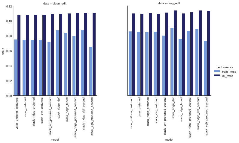
# compare clean and edit performance for train and cv error
plot_model_comp(ens_comp_df.head(10), col='performance', hue='data',
                kind='bar', palette=perf_palette)
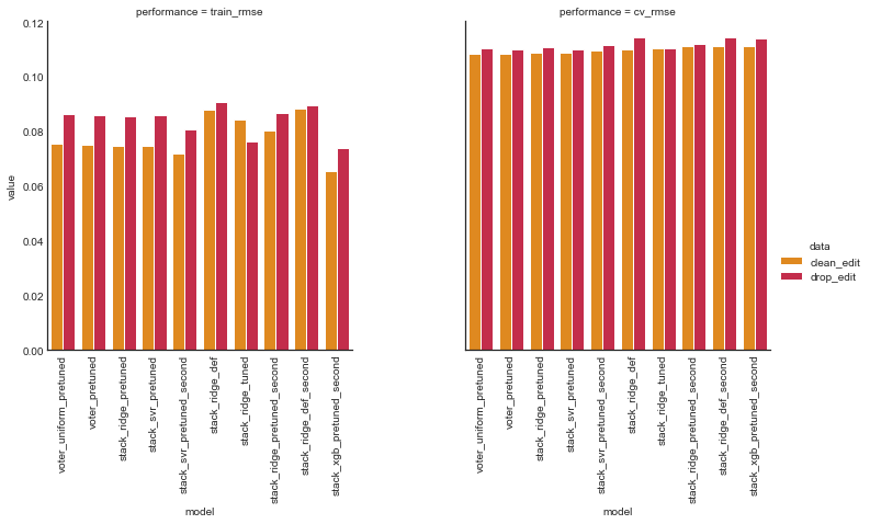
Overall, ensembles with pretuned base models performed better than those that were tuned all at once. Voting ensembles with pretuned bases and stack ensembles with ridge and support vector meta models were top models for both data sets.
# pickle tuned parameters
pickle_to_file(ensembles, '../training/ens_tuned_params.pkl')
Predict and Evaluate
To check our test prediction performance we need to submit to Kaggle. We’ll submit predictions for the top five ensemble models for both versions of the data (clean_edit and drop_edit) and report them here.
# save top 5 models from both data sets
save_top_model_predictions(ensembles=ensembles, ens_comp_df=ens_comp_df,
               data_name='clean_edit', model_data=model_data,
               num_models=5, save_path='../submissions')

save_top_model_predictions(ensembles=ensembles, ens_comp_df=ens_comp_df,
               data_name='drop_edit', model_data=model_data,
               num_models=5, save_path='../submissions')
# Enter results of Kaggle submissions
test_comp_df = test_comp(ens_comp_df)
test_comp_df.loc['stack_ridge_pretuned_drop_edit'] = 0.12297
test_comp_df.loc['voter_uniform_pretuned_drop_edit'] = 0.12307
test_comp_df.loc['stack_ridge_tuned_drop_edit'] = 0.12132
test_comp_df.loc['voter_pretuned_drop_edit'] = 0.12299
test_comp_df.loc['stack_svr_pretuned_drop_edit'] = 0.12329
test_comp_df.loc['stack_svr_pretuned_second_clean_edit'] = 0.12299
test_comp_df.loc['stack_svr_pretuned_clean_edit'] = 0.12192
test_comp_df.loc['stack_ridge_pretuned_clean_edit'] = 0.12203
test_comp_df.loc['voter_pretuned_clean_edit'] = 0.12192
test_comp_df.loc['voter_uniform_pretuned_clean_edit'] = 0.12193
test_comp_df.sort_values(by='test_rmse')
| test_rmse | |
|---|---|
| stack_ridge_tuned_drop_edit | 0.12132 |
| voter_pretuned_clean_edit | 0.12192 |
| stack_svr_pretuned_clean_edit | 0.12192 |
| voter_uniform_pretuned_clean_edit | 0.12193 |
| stack_ridge_pretuned_clean_edit | 0.12203 |
| stack_ridge_pretuned_drop_edit | 0.12297 |
| stack_svr_pretuned_second_clean_edit | 0.12299 |
| voter_pretuned_drop_edit | 0.12299 |
| voter_uniform_pretuned_drop_edit | 0.12307 |
| stack_svr_pretuned_drop_edit | 0.12329 |
Per Kaggle, “submissions are evaluated on Root-Mean-Squared-Error (RMSE) between the logarithm of the predicted value and the logarithm of the observed sales price”. That is submission scores are
It follows that we can identify
with the error in this case, and thus the values in test_comp_df as point estimates for each model.
# mean test_rmse
test_comp_df.mean()
test_rmse    0.122443
dtype: float64
# std dev test rmse
test_comp_df.std()
test_rmse    0.000685
dtype: float64
To get a better sense of our model performances, we can consider average test error as a point estimate . It’s unclear from the instructions (or discussion) which logarithm base was used, but assuming it’s natural log, this yields