Ames Housing Data Processing, analysis and predictive modeling
Exploratory analysis
In a previous notebook, we processed and cleaned the Ames housing dataset. In this notebook, we focus on exploring the variables and the relationships among them. In a later notebook we’ll model and predict sale prices.
Contents
Setup
# standard imports
%matplotlib inline
import matplotlib.pyplot as plt
import warnings
import scipy.stats as ss
import sys
import os

# add parent directory for importing custom classes
pardir = os.path.abspath(os.path.join(os.getcwd(), os.pardir))
sys.path.append(pardir)

# add root site-packages directory to workaround pyitlib pip install issue
sys.path.append('/Users/home/anaconda3/lib/python3.7/site-packages')

# custom classes
from codes.process import DataDescription
from codes.explore import *

# notebook settings
warnings.filterwarnings('ignore')
plt.style.use('seaborn-white')
sns.set_style('white')
Load and inspect data
data_dir = '../data'
file_names = ['orig.csv', 'clean.csv']
hp_data = load_datasets(data_dir, file_names)
orig, clean = (hp_data.dfs['orig'], hp_data.dfs['clean'])
We have 2 versions of the dataset here (created in a previous notebook)
origis the original dataset with no preprocessingcleanis the preprocessed dataset, with problematic variables and observations dropped and missing values imputed
. In this notebook we’ll primarily be working with the cleaned dataset
clean.data.head()
| MSSubClass | MSZoning | LotFrontage | LotArea | Street | LotShape | LandContour | Utilities | LotConfig | LandSlope | ... | ScreenPorch | PoolArea | PoolQC | Fence | MiscVal | MoSold | YrSold | SaleType | SaleCondition | SalePrice | ||
|---|---|---|---|---|---|---|---|---|---|---|---|---|---|---|---|---|---|---|---|---|---|---|
| Id | ||||||||||||||||||||||
| train | 1 | 60 | RL | 65.0 | 8450.0 | Pave | 0 | Lvl | 3 | Inside | 0 | ... | 0.0 | 0.0 | 0 | 0 | 0.0 | 2 | 2008 | WD | Normal | 208500.0 |
| 2 | 20 | RL | 80.0 | 9600.0 | Pave | 0 | Lvl | 3 | FR2 | 0 | ... | 0.0 | 0.0 | 0 | 0 | 0.0 | 5 | 2007 | WD | Normal | 181500.0 | |
| 3 | 60 | RL | 68.0 | 11250.0 | Pave | 1 | Lvl | 3 | Inside | 0 | ... | 0.0 | 0.0 | 0 | 0 | 0.0 | 9 | 2008 | WD | Normal | 223500.0 | |
| 4 | 70 | RL | 60.0 | 9550.0 | Pave | 1 | Lvl | 3 | Corner | 0 | ... | 0.0 | 0.0 | 0 | 0 | 0.0 | 2 | 2006 | WD | Abnorml | 140000.0 | |
| 5 | 60 | RL | 84.0 | 14260.0 | Pave | 1 | Lvl | 3 | FR2 | 0 | ... | 0.0 | 0.0 | 0 | 0 | 0.0 | 12 | 2008 | WD | Normal | 250000.0 |
5 rows × 78 columns
clean.data.info()
<class 'pandas.core.frame.DataFrame'>
MultiIndex: 2916 entries, (train, 1) to (test, 2919)
Data columns (total 78 columns):
MSSubClass       2916 non-null category
MSZoning         2916 non-null category
LotFrontage      2916 non-null float64
LotArea          2916 non-null float64
Street           2916 non-null category
LotShape         2916 non-null int64
LandContour      2916 non-null category
Utilities        2916 non-null int64
LotConfig        2916 non-null category
LandSlope        2916 non-null int64
Neighborhood     2916 non-null category
Condition1       2916 non-null category
Condition2       2916 non-null category
BldgType         2916 non-null category
HouseStyle       2916 non-null category
OverallQual      2916 non-null int64
OverallCond      2916 non-null int64
YearBuilt        2916 non-null float64
YearRemodAdd     2916 non-null float64
RoofStyle        2916 non-null category
RoofMatl         2916 non-null category
Exterior1st      2916 non-null category
Exterior2nd      2916 non-null category
MasVnrType       2916 non-null category
MasVnrArea       2916 non-null float64
ExterQual        2916 non-null int64
ExterCond        2916 non-null int64
Foundation       2916 non-null category
BsmtQual         2916 non-null int64
BsmtCond         2916 non-null int64
BsmtExposure     2916 non-null int64
BsmtFinType1     2916 non-null int64
BsmtFinSF1       2916 non-null float64
BsmtFinType2     2916 non-null int64
BsmtFinSF2       2916 non-null float64
BsmtUnfSF        2916 non-null float64
TotalBsmtSF      2916 non-null float64
Heating          2916 non-null category
HeatingQC        2916 non-null int64
CentralAir       2916 non-null category
Electrical       2916 non-null category
1stFlrSF         2916 non-null float64
2ndFlrSF         2916 non-null float64
LowQualFinSF     2916 non-null float64
GrLivArea        2916 non-null float64
BsmtFullBath     2916 non-null int64
BsmtHalfBath     2916 non-null int64
FullBath         2916 non-null int64
HalfBath         2916 non-null int64
BedroomAbvGr     2916 non-null int64
KitchenAbvGr     2916 non-null int64
KitchenQual      2916 non-null int64
TotRmsAbvGrd     2916 non-null int64
Functional       2916 non-null int64
Fireplaces       2916 non-null int64
FireplaceQu      2916 non-null int64
GarageType       2916 non-null category
GarageYrBlt      2916 non-null float64
GarageFinish     2916 non-null int64
GarageCars       2916 non-null int64
GarageArea       2916 non-null float64
GarageQual       2916 non-null int64
GarageCond       2916 non-null int64
PavedDrive       2916 non-null int64
WoodDeckSF       2916 non-null float64
OpenPorchSF      2916 non-null float64
EnclosedPorch    2916 non-null float64
3SsnPorch        2916 non-null float64
ScreenPorch      2916 non-null float64
PoolArea         2916 non-null float64
PoolQC           2916 non-null int64
Fence            2916 non-null int64
MiscVal          2916 non-null float64
MoSold           2916 non-null int64
YrSold           2916 non-null int64
SaleType         2916 non-null category
SaleCondition    2916 non-null category
SalePrice        1457 non-null float64
dtypes: category(22), float64(23), int64(33)
memory usage: 1.3+ MB
The response variable SalePrice
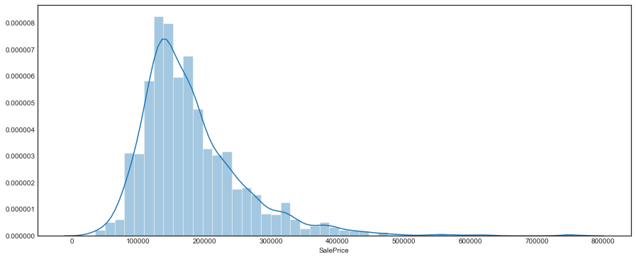
First let’s look at the distribution of SalePrice, the variable we’ll later be interested in predicting.
sale_price = clean.data.loc['train', :]['SalePrice']
plt.figure(figsize=(15, 6))
sns.distplot(sale_price)
<matplotlib.axes._subplots.AxesSubplot at 0x11c407cc0>
plt.figure(figsize=(15, 6))
sns.swarmplot(sale_price)
<matplotlib.axes._subplots.AxesSubplot at 0x11c580d68>
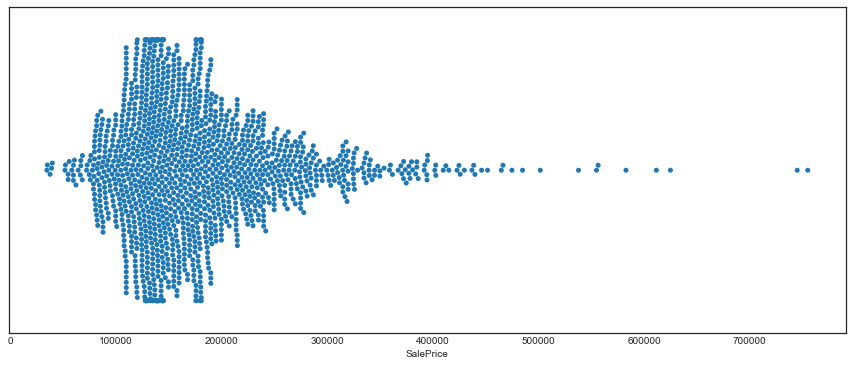
The distribution is positively skewed, with a long right tail. There are two observations with SalePrice > 700000, and with a good separation from the rest of the points.
# check skewness of SalePrice
sale_price.skew()
1.88374941136315
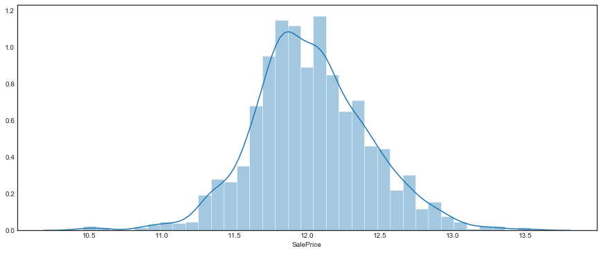
Testing log-normality
The distribution looks like it may be approximately log-normal, let’s check this
# distribution of log(SalePrice)
plt.figure(figsize=(15, 6))
sns.distplot(np.log(sale_price))
<matplotlib.axes._subplots.AxesSubplot at 0x11c733b00>
QQ-plot
# lognormal QQ plot
plt.figure(figsize=(8, 8))
# standard deviation of log is the shape parameter
s = np.log(sale_price).std()
lognorm = ss.lognorm(s)
ss.probplot(sale_price, dist=lognorm, plot=plt)
plt.show()
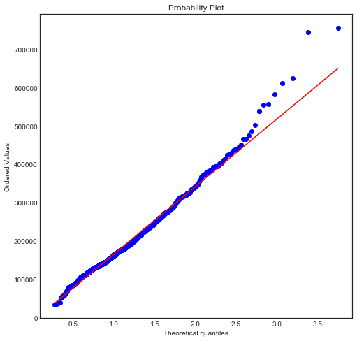
The distribution appears to be approxiately log-normal, although the QQ plot shows the right tail is a bit longer than expected, and the two observations with highest SalePrice are much higher than expected.
Kolmogorov - Smirnov test
This is a non-parametric test for comparing distributions. We’ll use scipy.stats implementation
ss.kstest(sale_price, lognorm.cdf)
KstestResult(statistic=1.0, pvalue=0.0)
This test conclusively rejects the null hypothesis that the distribution of SalePrice is lognormal. Nevertheless, the plots indicate that log-normality is perhaps a usefull approximation. Moreover, log(SalePrice) may be more useful than SalePrice for prediction purposes, given the symmetry of its distribution.
Categorical variables
First we look at all categorical variables, that is, all discrete variables with no ordering on the values. In our cleaned dataframe these are all the columns with category dtype
# dataframe of categorical variables
cats = HPDataFramePlus(data=clean.data.select_dtypes('category'))
cats.data.head()
| MSSubClass | MSZoning | Street | LandContour | LotConfig | Neighborhood | Condition1 | Condition2 | BldgType | HouseStyle | ... | Exterior1st | Exterior2nd | MasVnrType | Foundation | Heating | CentralAir | Electrical | GarageType | SaleType | SaleCondition | ||
|---|---|---|---|---|---|---|---|---|---|---|---|---|---|---|---|---|---|---|---|---|---|---|
| Id | ||||||||||||||||||||||
| train | 1 | 60 | RL | Pave | Lvl | Inside | CollgCr | Norm | Norm | 1Fam | 2Story | ... | VinylSd | VinylSd | BrkFace | PConc | GasA | Y | SBrkr | Attchd | WD | Normal |
| 2 | 20 | RL | Pave | Lvl | FR2 | Veenker | Feedr | Norm | 1Fam | 1Story | ... | MetalSd | MetalSd | None | CBlock | GasA | Y | SBrkr | Attchd | WD | Normal | |
| 3 | 60 | RL | Pave | Lvl | Inside | CollgCr | Norm | Norm | 1Fam | 2Story | ... | VinylSd | VinylSd | BrkFace | PConc | GasA | Y | SBrkr | Attchd | WD | Normal | |
| 4 | 70 | RL | Pave | Lvl | Corner | Crawfor | Norm | Norm | 1Fam | 2Story | ... | Wd Sdng | Wd Shng | None | BrkTil | GasA | Y | SBrkr | Detchd | WD | Abnorml | |
| 5 | 60 | RL | Pave | Lvl | FR2 | NoRidge | Norm | Norm | 1Fam | 2Story | ... | VinylSd | VinylSd | BrkFace | PConc | GasA | Y | SBrkr | Attchd | WD | Normal |
5 rows × 22 columns
# print description of categorical variables
desc = DataDescription('../data/data_description.txt')
cats.desc = desc
cats.print_desc(cols=cats.data.columns)
MSSubClass: Identifies the type of dwelling involved in the sale.

	 20 - 1-STORY 1946 & NEWER ALL STYLES
	 30 - 1-STORY 1945 & OLDER
	 40 - 1-STORY W/FINISHED ATTIC ALL AGES
	 45 - 1-1/2 STORY - UNFINISHED ALL AGES
	 50 - 1-1/2 STORY FINISHED ALL AGES
	 60 - 2-STORY 1946 & NEWER
	 70 - 2-STORY 1945 & OLDER
	 75 - 2-1/2 STORY ALL AGES
	 80 - SPLIT OR MULTI-LEVEL
	 85 - SPLIT FOYER
	 90 - DUPLEX - ALL STYLES AND AGES
	 120 - 1-STORY PUD (Planned Unit Development) - 1946 & NEWER
	 150 - 1-1/2 STORY PUD - ALL AGES
	 160 - 2-STORY PUD - 1946 & NEWER
	 180 - PUD - MULTILEVEL - INCL SPLIT LEV/FOYER
	 190 - 2 FAMILY CONVERSION - ALL STYLES AND AGES


MSZoning: Identifies the general zoning classification of the sale.

	 A - Agriculture
	 C - Commercial
	 FV - Floating Village Residential
	 I - Industrial
	 RH - Residential High Density
	 RL - Residential Low Density
	 RP - Residential Low Density Park
	 RM - Residential Medium Density


Street: Type of road access to property

	 Grvl - Gravel
	 Pave - Paved


LandContour: Flatness of the property

	 Lvl - Near Flat/Level
	 Bnk - Banked - Quick and significant rise from street grade to building
	 HLS - Hillside - Significant slope from side to side
	 Low - Depression


LotConfig: Lot configuration

	 Inside - Inside lot
	 Corner - Corner lot
	 CulDSac - Cul-de-sac
	 FR2 - Frontage on 2 sides of property
	 FR3 - Frontage on 3 sides of property


Neighborhood: Physical locations within Ames city limits

	 Blmngtn - Bloomington Heights
	 Blueste - Bluestem
	 BrDale - Briardale
	 BrkSide - Brookside
	 ClearCr - Clear Creek
	 CollgCr - College Creek
	 Crawfor - Crawford
	 Edwards - Edwards
	 Gilbert - Gilbert
	 IDOTRR - Iowa DOT and Rail Road
	 MeadowV - Meadow Village
	 Mitchel - Mitchell
	 Names - North Ames
	 NoRidge - Northridge
	 NPkVill - Northpark Villa
	 NridgHt - Northridge Heights
	 NWAmes - Northwest Ames
	 OldTown - Old Town
	 SWISU - South & West of Iowa State University
	 Sawyer - Sawyer
	 SawyerW - Sawyer West
	 Somerst - Somerset
	 StoneBr - Stone Brook
	 Timber - Timberland
	 Veenker - Veenker


Condition1: Proximity to various conditions

	 Artery - Adjacent to arterial street
	 Feedr - Adjacent to feeder street
	 Norm - Normal
	 RRNn - Within 200' of North-South Railroad
	 RRAn - Adjacent to North-South Railroad
	 PosN - Near positive off-site feature--park, greenbelt, etc.
	 PosA - Adjacent to postive off-site feature
	 RRNe - Within 200' of East-West Railroad
	 RRAe - Adjacent to East-West Railroad


Condition2: Proximity to various conditions (if more than one is present)

	 Artery - Adjacent to arterial street
	 Feedr - Adjacent to feeder street
	 Norm - Normal
	 RRNn - Within 200' of North-South Railroad
	 RRAn - Adjacent to North-South Railroad
	 PosN - Near positive off-site feature--park, greenbelt, etc.
	 PosA - Adjacent to postive off-site feature
	 RRNe - Within 200' of East-West Railroad
	 RRAe - Adjacent to East-West Railroad


BldgType: Type of dwelling

	 1Fam - Single-family Detached
	 2FmCon - Two-family Conversion; originally built as one-family dwelling
	 Duplx - Duplex
	 TwnhsE - Townhouse End Unit
	 TwnhsI - Townhouse Inside Unit


HouseStyle: Style of dwelling

	 1Story - One story
	 1.5Fin - One and one-half story: 2nd level finished
	 1.5Unf - One and one-half story: 2nd level unfinished
	 2Story - Two story
	 2.5Fin - Two and one-half story: 2nd level finished
	 2.5Unf - Two and one-half story: 2nd level unfinished
	 SFoyer - Split Foyer
	 SLvl - Split Level


RoofStyle: Type of roof

	 Flat - Flat
	 Gable - Gable
	 Gambrel - Gabrel (Barn)
	 Hip - Hip
	 Mansard - Mansard
	 Shed - Shed


RoofMatl: Roof material

	 ClyTile - Clay or Tile
	 CompShg - Standard (Composite) Shingle
	 Membran - Membrane
	 Metal - Metal
	 Roll - Roll
	 Tar&Grv - Gravel & Tar
	 WdShake - Wood Shakes
	 WdShngl - Wood Shingles


Exterior1st: Exterior covering on house

	 AsbShng - Asbestos Shingles
	 AsphShn - Asphalt Shingles
	 BrkComm - Brick Common
	 BrkFace - Brick Face
	 CBlock - Cinder Block
	 CemntBd - Cement Board
	 HdBoard - Hard Board
	 ImStucc - Imitation Stucco
	 MetalSd - Metal Siding
	 Other - Other
	 Plywood - Plywood
	 PreCast - PreCast
	 Stone - Stone
	 Stucco - Stucco
	 VinylSd - Vinyl Siding
	 Wd - Wood Siding
	 WdShing - Wood Shingles


Exterior2nd: Exterior covering on house (if more than one material)

	 AsbShng - Asbestos Shingles
	 AsphShn - Asphalt Shingles
	 BrkComm - Brick Common
	 BrkFace - Brick Face
	 CBlock - Cinder Block
	 CemntBd - Cement Board
	 HdBoard - Hard Board
	 ImStucc - Imitation Stucco
	 MetalSd - Metal Siding
	 Other - Other
	 Plywood - Plywood
	 PreCast - PreCast
	 Stone - Stone
	 Stucco - Stucco
	 VinylSd - Vinyl Siding
	 Wd - Wood Siding
	 WdShing - Wood Shingles


MasVnrType: Masonry veneer type

	 BrkCmn - Brick Common
	 BrkFace - Brick Face
	 CBlock - Cinder Block
	 None - None
	 Stone - Stone


Foundation: Type of foundation

	 BrkTil - Brick & Tile
	 CBlock - Cinder Block
	 PConc - Poured Contrete
	 Slab - Slab
	 Stone - Stone
	 Wood - Wood


Heating: Type of heating

	 Floor - Floor Furnace
	 GasA - Gas forced warm air furnace
	 GasW - Gas hot water or steam heat
	 Grav - Gravity furnace
	 OthW - Hot water or steam heat other than gas
	 Wall - Wall furnace


CentralAir: Central air conditioning

	 N - No
	 Y - Yes


Electrical: Electrical system

	 SBrkr - Standard Circuit Breakers & Romex
	 FuseA - Fuse Box over 60 AMP and all Romex wiring (Average)
	 FuseF - 60 AMP Fuse Box and mostly Romex wiring (Fair)
	 FuseP - 60 AMP Fuse Box and mostly knob & tube wiring (poor)
	 Mix - Mixed


GarageType: Garage location

	 2Types - More than one type of garage
	 Attchd - Attached to home
	 Basment - Basement Garage
	 BuiltIn - Built-In (Garage part of house - typically has room above garage)
	 CarPort - Car Port
	 Detchd - Detached from home
	 NA - No Garage


SaleType: Type of sale

	 WD - Warranty Deed - Conventional
	 CWD - Warranty Deed - Cash
	 VWD - Warranty Deed - VA Loan
	 New - Home just constructed and sold
	 COD - Court Officer Deed/Estate
	 Con - Contract 15% Down payment regular terms
	 ConLw - Contract Low Down payment and low interest
	 ConLI - Contract Low Interest
	 ConLD - Contract Low Down
	 Oth - Other


SaleCondition: Condition of sale

	 Normal - Normal Sale
	 Abnorml - Abnormal Sale -  trade, foreclosure, short sale
	 AdjLand - Adjoining Land Purchase
	 Alloca - Allocation - two linked properties with separate deeds, typically condo with a garage unit
	 Family - Sale between family members
	 Partial - Home was not completed when last assessed (associated with New Homes)
Distributions of categorical variables
# plot distributions of categorical variables
plot_discrete_dists(nrows=8, ncols=3, data=cats.data, figsize=(15, 30))
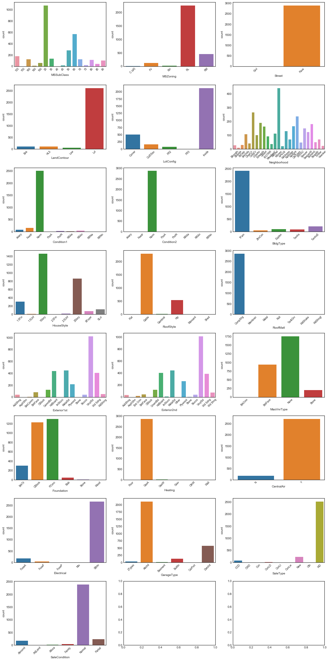
Some of these variables have highly unbalanced distributions. We’ll look for the most extremely unbalanced
# print distributions of categorical variables with more 90% concentration at single value
unbal_cat_cols = print_unbal_dists(data=cats.data, bal_threshold=0.9)
Pave    0.995885
Grvl    0.004115
Name: Street, dtype: float64

Norm      0.990055
Feedr     0.004458
Artery    0.001715
PosA      0.001372
PosN      0.001029
RRNn      0.000686
RRAn      0.000343
RRAe      0.000343
Name: Condition2, dtype: float64

CompShg    0.985940
Tar&Grv    0.007545
WdShake    0.003086
WdShngl    0.002401
Roll       0.000343
Metal      0.000343
Membran    0.000343
Name: RoofMatl, dtype: float64

GasA     0.984568
GasW     0.009259
Grav     0.003086
Wall     0.002058
OthW     0.000686
Floor    0.000343
Name: Heating, dtype: float64

Y    0.932785
N    0.067215
Name: CentralAir, dtype: float64

SBrkr    0.915295
FuseA    0.064472
FuseF    0.017147
FuseP    0.002743
Mix      0.000343
Name: Electrical, dtype: float64
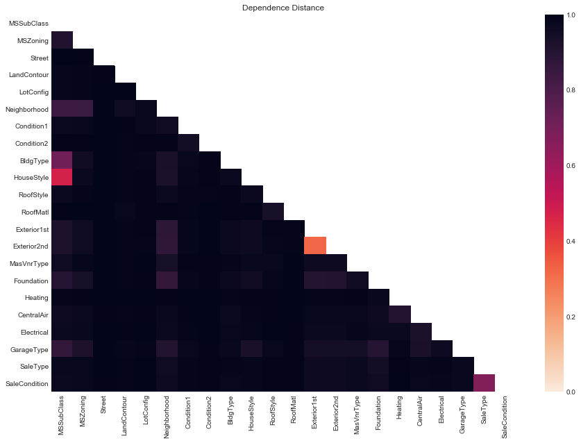
Relationships among categorical variables
One often speaks loosely of “correlation” among variables to refer to statistical dependence. There are various measures of dependence, but here we rely on an information theoretic measure known as the variation of information. We discuss this measure briefly
The function
where is the joint entropy and the mutual information, defines a metric on a set of discrete random variables. Note that
which is sometimes called the “variation of information”. One can normalize to get a standardized variation of information
i.e. . Since is a metric, iff Furthermore, if and only if if and only if are independendent. So we can take as a “dependence distance”. The closer a variable is to , the more it depends on .
Of course, we don’t know the true distributions of the random variables in this data set, but the sample size is large enough that the sample distributions should be a good approximation.
We’ll look at the dependence distance among variables with feature selection in mind, namely the possibility of removing redundant variables.
# Get dataframe of dependence distances of categorical variables
cats_data_num = num_enc(data=cats.data)
cats_D_dep_df = D_dep(data=cats_data_num)
# plot all dependence distances
plot_D_dep(cats_D_dep_df, figsize=(15, 10))
# plot dependence distances less than 0.8
plot_low_D_dep(D_dep_df=cats_D_dep_df, D_threshold=0.8, figsize=(13, 8))
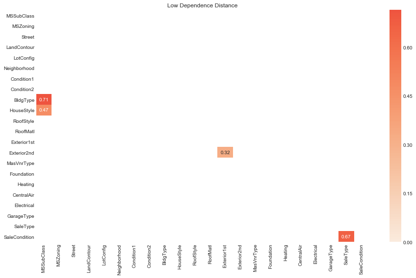
# rank categorical variables by dependence distance
rank_pairs_by_D(D_dep_df=cats_D_dep_df, D_threshold=0.8)
| var1 | var2 | D | |
|---|---|---|---|
| 1 | Exterior1st | Exterior2nd | 0.322737 |
| 2 | MSSubClass | HouseStyle | 0.472661 |
| 3 | SaleType | SaleCondition | 0.667950 |
| 4 | MSSubClass | BldgType | 0.714236 |
Notable pairs of distinct variables with low dependence distance are
Exterior1standExterior2ndhave the lowest dependence distance (). Their distributions are very similar and they have the same values. It probably makes more sense to think of them as close to identically distributed.MSSubclassandHouseStylehave the next lowest (). Inspecting their descriptions above we see that they have very similar categories, so they are measuring very similar things.BldgTypeandMSSubclass() are similar.MSSubclassandNeighborhood() are perhaps the first interesting pair in that they are measuring different things. We can imagine that the association between these two variables is somewhat strong – it makes sense that the size/age/type of house would be related to the neighborhood. Similarly,Exterior1st,Exterior2nd,MSZoning,Foundationalso have strong associations withNeighborhood.SaleConditionandSaleType() are also unsurprisingly associated.
Relationships between categoricals and SalePrice
Given that SalePrice seemed to be well-approximated by a log-normal distribution, we’ll measure dependence with log_SalePrice.
cats_data_num['log_SalePrice'] = np.log(clean.data['SalePrice'])
cats_data_num['log_SalePrice']
       Id
train  1       12.247694
       2       12.109011
       3       12.317167
       4       11.849398
       5       12.429216
                 ...
test   2915          NaN
       2916          NaN
       2917          NaN
       2918          NaN
       2919          NaN
Name: log_SalePrice, Length: 2916, dtype: float64
To visualize the relationship between the categorical variables and the response, we’ll look at the distributions of log_SalePrice over the values of the variables.
# violin plots of categorical variables vs. response
plot_violin_plots(nrows=8, ncols=3, data=cats_data_num, response='log_SalePrice', figsize=(15, 30))
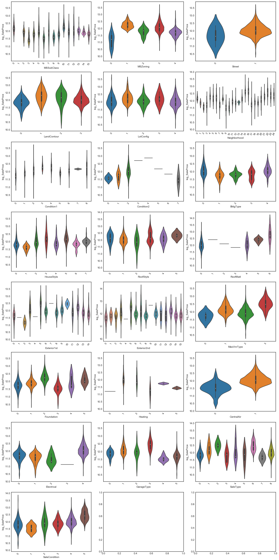
Note that horizontal lines for variable values in the violin plots indicate less than 5 observations having that value
From these plots, it’s difficult to determine with accuracy for which variables the distribution of log_SalePrice doesn’t seem to vary greatly across values (and hence are of low dependence and thus low predictive value). The dependence distance between the variables and log_SalePrice will provide additional information.
# rank categorical variables by dependence distance from response
D_dep_response(cats_data_num, 'log_SalePrice').sort_values(by='D').T
| Neighborhood | MSSubClass | Exterior2nd | Exterior1st | HouseStyle | Foundation | GarageType | MasVnrType | SaleCondition | LotConfig | ... | Condition1 | BldgType | RoofStyle | LandContour | Electrical | CentralAir | Heating | RoofMatl | Condition2 | Street | |
|---|---|---|---|---|---|---|---|---|---|---|---|---|---|---|---|---|---|---|---|---|---|
| D | 0.713181 | 0.813289 | 0.831957 | 0.838796 | 0.894477 | 0.901514 | 0.919312 | 0.924422 | 0.926004 | 0.929782 | ... | 0.937908 | 0.938181 | 0.947682 | 0.956498 | 0.966163 | 0.973683 | 0.990074 | 0.990213 | 0.991566 | 0.996507 |
1 rows × 22 columns
The lower the dependence distance here, the better assocation with the response, hence the better the potential predictive value.
In particular, given how unbalanced their distributions are, it’s perhaps not too surprising to see RoofStyle, LandContour, Electrical and CentralAir all have such high dependence distance,
Ordinal variables
Now we’ll investigate ordinal variables, that is discrete variables with an ordering. In our cleaned dataframe these are variables with int64 dtype
# dataframe of ordinal variables
ords = HPDataFramePlus(data=clean.data.select_dtypes('int64'))
ords.data.head()
| LotShape | Utilities | LandSlope | OverallQual | OverallCond | ExterQual | ExterCond | BsmtQual | BsmtCond | BsmtExposure | ... | FireplaceQu | GarageFinish | GarageCars | GarageQual | GarageCond | PavedDrive | PoolQC | Fence | MoSold | YrSold | ||
|---|---|---|---|---|---|---|---|---|---|---|---|---|---|---|---|---|---|---|---|---|---|---|
| Id | ||||||||||||||||||||||
| train | 1 | 0 | 3 | 0 | 7 | 5 | 2 | 3 | 3 | 3 | 1 | ... | 0 | 2 | 2 | 3 | 3 | 2 | 0 | 0 | 2 | 2008 |
| 2 | 0 | 3 | 0 | 6 | 8 | 1 | 3 | 3 | 3 | 4 | ... | 3 | 2 | 2 | 3 | 3 | 2 | 0 | 0 | 5 | 2007 | |
| 3 | 1 | 3 | 0 | 7 | 5 | 2 | 3 | 3 | 3 | 2 | ... | 3 | 2 | 2 | 3 | 3 | 2 | 0 | 0 | 9 | 2008 | |
| 4 | 1 | 3 | 0 | 7 | 5 | 1 | 3 | 2 | 4 | 1 | ... | 4 | 1 | 3 | 3 | 3 | 2 | 0 | 0 | 2 | 2006 | |
| 5 | 1 | 3 | 0 | 8 | 5 | 2 | 3 | 3 | 3 | 3 | ... | 3 | 2 | 3 | 3 | 3 | 2 | 0 | 0 | 12 | 2008 |
5 rows × 33 columns
ords.data.info()
<class 'pandas.core.frame.DataFrame'>
MultiIndex: 2916 entries, (train, 1) to (test, 2919)
Data columns (total 33 columns):
LotShape        2916 non-null int64
Utilities       2916 non-null int64
LandSlope       2916 non-null int64
OverallQual     2916 non-null int64
OverallCond     2916 non-null int64
ExterQual       2916 non-null int64
ExterCond       2916 non-null int64
BsmtQual        2916 non-null int64
BsmtCond        2916 non-null int64
BsmtExposure    2916 non-null int64
BsmtFinType1    2916 non-null int64
BsmtFinType2    2916 non-null int64
HeatingQC       2916 non-null int64
BsmtFullBath    2916 non-null int64
BsmtHalfBath    2916 non-null int64
FullBath        2916 non-null int64
HalfBath        2916 non-null int64
BedroomAbvGr    2916 non-null int64
KitchenAbvGr    2916 non-null int64
KitchenQual     2916 non-null int64
TotRmsAbvGrd    2916 non-null int64
Functional      2916 non-null int64
Fireplaces      2916 non-null int64
FireplaceQu     2916 non-null int64
GarageFinish    2916 non-null int64
GarageCars      2916 non-null int64
GarageQual      2916 non-null int64
GarageCond      2916 non-null int64
PavedDrive      2916 non-null int64
PoolQC          2916 non-null int64
Fence           2916 non-null int64
MoSold          2916 non-null int64
YrSold          2916 non-null int64
dtypes: int64(33)
memory usage: 783.3+ KB
We’ll print the description of all variables, however note that the print description contains the original value for the variables, while the cleaned dataframe clean contains the numerically encoded values
# print description of ordinal variables
ords.desc = desc
ords.print_desc(cols=ords.data.columns)
LotShape: General shape of property

	 Reg - Regular
	 IR1 - Slightly irregular
	 IR2 - Moderately Irregular
	 IR3 - Irregular


Utilities: Type of utilities available

	 AllPub - All public Utilities (E,G,W,& S)
	 NoSewr - Electricity, Gas, and Water (Septic Tank)
	 NoSeWa - Electricity and Gas Only
	 ELO - Electricity only


LandSlope: Slope of property

	 Gtl - Gentle slope
	 Mod - Moderate Slope
	 Sev - Severe Slope


OverallQual: Rates the overall material and finish of the house

	 10 - Very Excellent
	 9 - Excellent
	 8 - Very Good
	 7 - Good
	 6 - Above Average
	 5 - Average
	 4 - Below Average
	 3 - Fair
	 2 - Poor
	 1 - Very Poor


OverallCond: Rates the overall condition of the house

	 10 - Very Excellent
	 9 - Excellent
	 8 - Very Good
	 7 - Good
	 6 - Above Average
	 5 - Average
	 4 - Below Average
	 3 - Fair
	 2 - Poor
	 1 - Very Poor


ExterQual: Evaluates the quality of the material on the exterior

	 Ex - Excellent
	 Gd - Good
	 TA - Average/Typical
	 Fa - Fair
	 Po - Poor


ExterCond: Evaluates the present condition of the material on the exterior

	 Ex - Excellent
	 Gd - Good
	 TA - Average/Typical
	 Fa - Fair
	 Po - Poor


BsmtQual: Evaluates the height of the basement

	 Ex - Excellent (100+ inches)
	 Gd - Good (90-99 inches)
	 TA - Typical (80-89 inches)
	 Fa - Fair (70-79 inches)
	 Po - Poor (<70 inches
	 NA - No Basement


BsmtCond: Evaluates the general condition of the basement

	 Ex - Excellent
	 Gd - Good
	 TA - Typical - slight dampness allowed
	 Fa - Fair - dampness or some cracking or settling
	 Po - Poor - Severe cracking, settling, or wetness
	 NA - No Basement


BsmtExposure: Refers to walkout or garden level walls

	 Gd - Good Exposure
	 Av - Average Exposure (split levels or foyers typically score average or above)
	 Mn - Mimimum Exposure
	 No - No Exposure
	 NA - No Basement


BsmtFinType1: Rating of basement finished area

	 GLQ - Good Living Quarters
	 ALQ - Average Living Quarters
	 BLQ - Below Average Living Quarters
	 Rec - Average Rec Room
	 LwQ - Low Quality
	 Unf - Unfinshed
	 NA - No Basement


BsmtFinType2: Rating of basement finished area (if multiple types)

	 GLQ - Good Living Quarters
	 ALQ - Average Living Quarters
	 BLQ - Below Average Living Quarters
	 Rec - Average Rec Room
	 LwQ - Low Quality
	 Unf - Unfinshed
	 NA - No Basement


HeatingQC: Heating quality and condition

	 Ex - Excellent
	 Gd - Good
	 TA - Average/Typical
	 Fa - Fair
	 Po - Poor


BsmtFullBath: Basement full bathrooms


BsmtHalfBath: Basement half bathrooms


FullBath: Full bathrooms above grade


HalfBath: Half baths above grade


BedroomAbvGr: Bedrooms above grade (does NOT include basement bedrooms)


KitchenAbvGr: Kitchens above grade


KitchenQual: Kitchen quality

	 Ex - Excellent
	 Gd - Good
	 TA - Typical/Average
	 Fa - Fair
	 Po - Poor


TotRmsAbvGrd: Total rooms above grade (does not include bathrooms)


Functional: Home functionality (Assume typical unless deductions are warranted)

	 Typ - Typical Functionality
	 Min1 - Minor Deductions 1
	 Min2 - Minor Deductions 2
	 Mod - Moderate Deductions
	 Maj1 - Major Deductions 1
	 Maj2 - Major Deductions 2
	 Sev - Severely Damaged
	 Sal - Salvage only


Fireplaces: Number of fireplaces


FireplaceQu: Fireplace quality

	 Ex - Excellent - Exceptional Masonry Fireplace
	 Gd - Good - Masonry Fireplace in main level
	 TA - Average - Prefabricated Fireplace in main living area or Masonry Fireplace in basement
	 Fa - Fair - Prefabricated Fireplace in basement
	 Po - Poor - Ben Franklin Stove
	 NA - No Fireplace


GarageFinish: Interior finish of the garage

	 Fin - Finished
	 RFn - Rough Finished
	 Unf - Unfinished
	 NA - No Garage


GarageCars: Size of garage in car capacity


GarageQual: Garage quality

	 Ex - Excellent
	 Gd - Good
	 TA - Typical/Average
	 Fa - Fair
	 Po - Poor
	 NA - No Garage


GarageCond: Garage condition

	 Ex - Excellent
	 Gd - Good
	 TA - Typical/Average
	 Fa - Fair
	 Po - Poor
	 NA - No Garage


PavedDrive: Paved driveway

	 Y - Paved
	 P - Partial Pavement
	 N - Dirt/Gravel


PoolQC: Pool quality

	 Ex - Excellent
	 Gd - Good
	 TA - Average/Typical
	 Fa - Fair
	 NA - No Pool


Fence: Fence quality

	 GdPrv - Good Privacy
	 MnPrv - Minimum Privacy
	 GdWo - Good Wood
	 MnWw - Minimum Wood/Wire
	 NA - No Fence


MoSold: Month Sold (MM)


YrSold: Year Sold (YYYY)
Distributions of ordinal variables
# plot distributions of ordinal variables
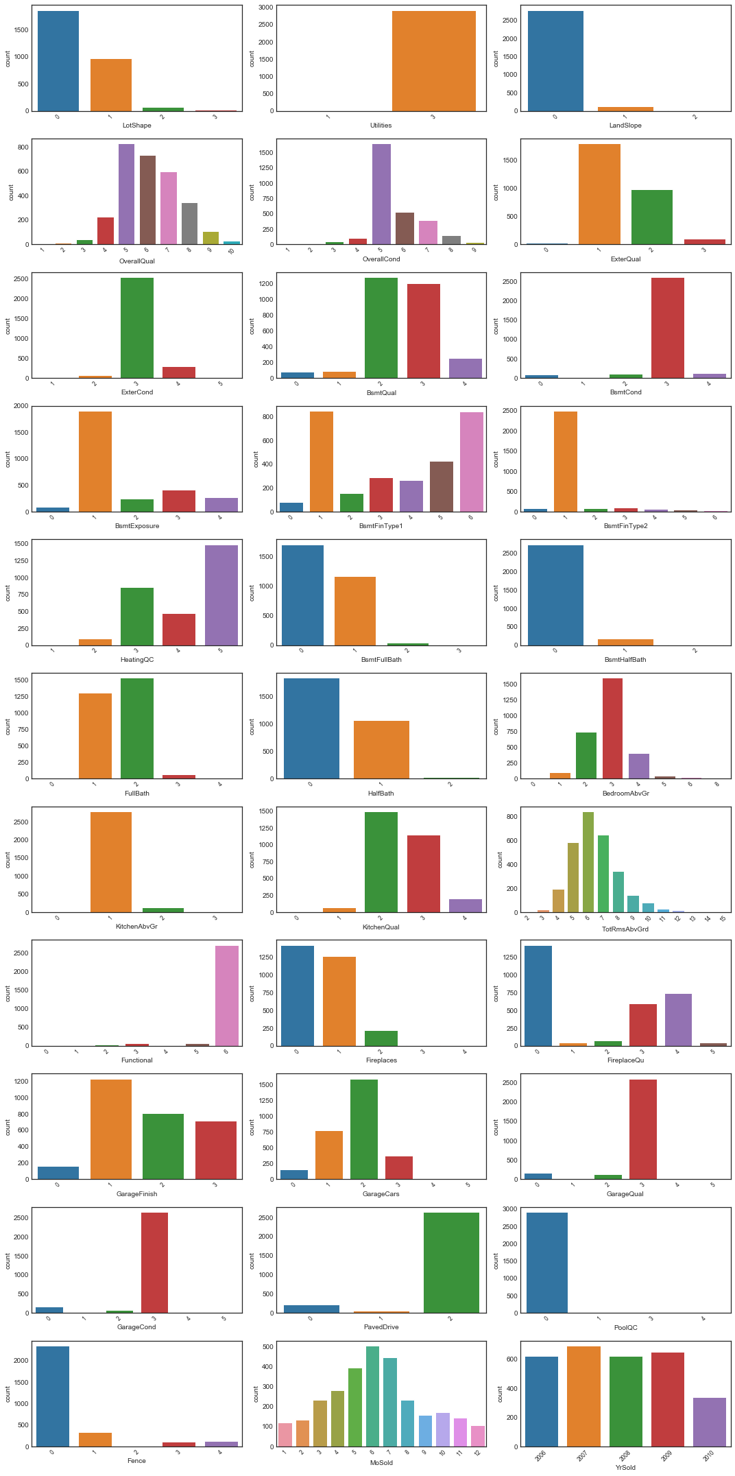
plot_discrete_dists(nrows=11, ncols=3, data=ords.data, figsize=(15, 30))
# look at most unbalanced distributions
unbal_ord_cols = print_unbal_dists(data=ords.data, bal_threshold=0.9)
3    0.999657
1    0.000343
Name: Utilities, dtype: float64

0    0.951989
1    0.042524
2    0.005487
Name: LandSlope, dtype: float64

0    0.939986
1    0.058642
2    0.001372
Name: BsmtHalfBath, dtype: float64

1    0.954047
2    0.044239
0    0.001029
3    0.000686
Name: KitchenAbvGr, dtype: float64

6    0.931756
3    0.024005
5    0.021948
2    0.012003
4    0.006516
1    0.003086
0    0.000686
Name: Functional, dtype: float64

3    0.909122
0    0.054527
2    0.025377
4    0.005144
1    0.004801
5    0.001029
Name: GarageCond, dtype: float64

2    0.904664
0    0.074074
1    0.021262
Name: PavedDrive, dtype: float64

0    0.996914
4    0.001372
3    0.001029
1    0.000686
Name: PoolQC, dtype: float64
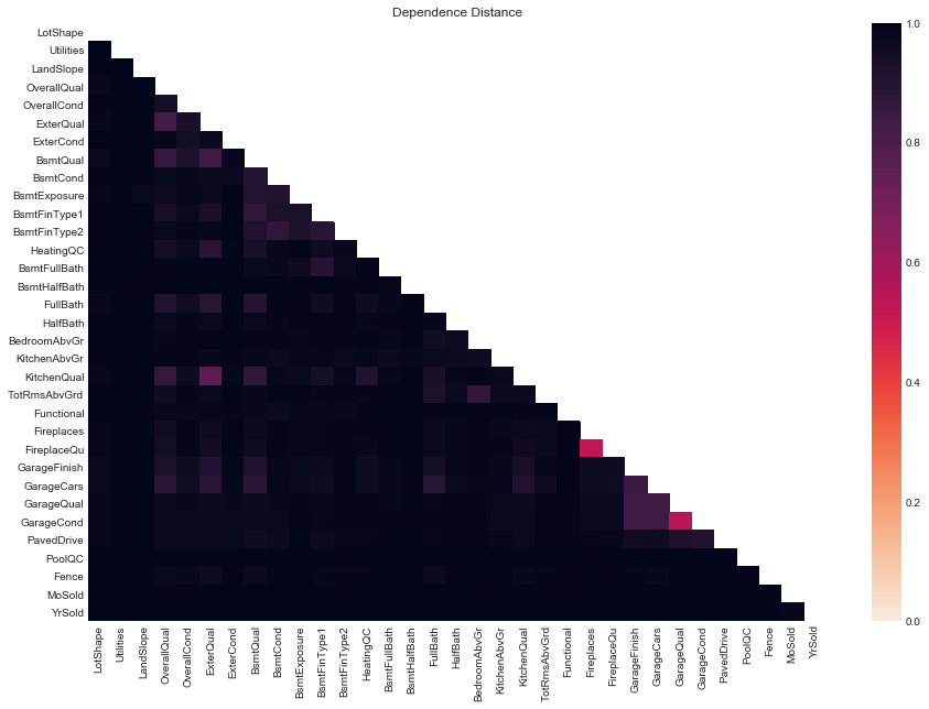
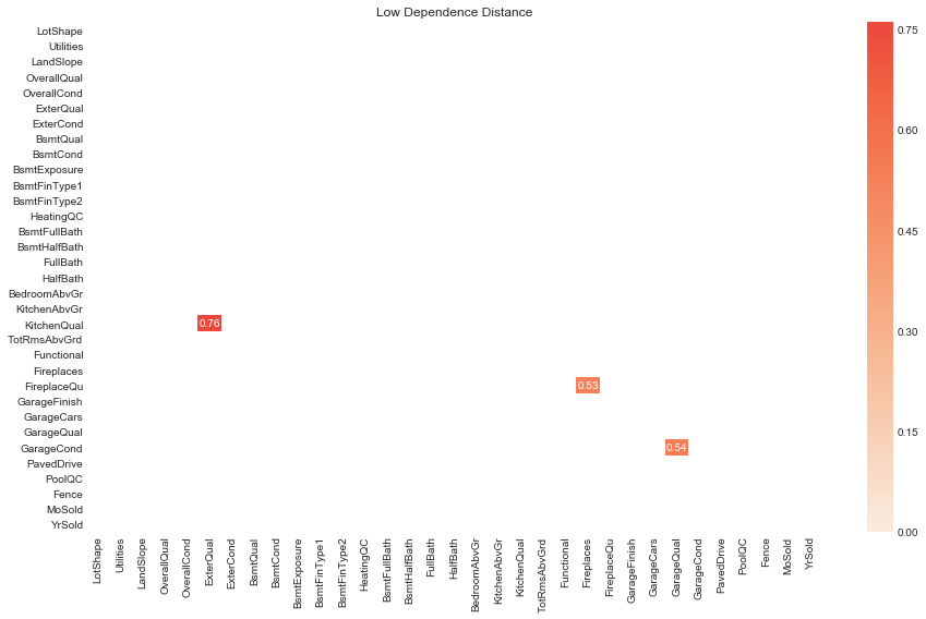
Relationships among ordinal variables
# get dataframe of dependence distances of ordinal variables
ords_D_dep_df = D_dep(ords.data)
# plot all dependence distances
plot_D_dep(D_dep_df=ords_D_dep_df, figsize=(15, 10))
# plot lower dependence distances of ordinal variables
plot_low_D_dep(D_dep_df=ords_D_dep_df, D_threshold=0.8, figsize=(13, 8))
# rank ordinals by low dependence distance
rank_pairs_by_D(D_dep_df=ords_D_dep_df, D_threshold=0.8)
| var1 | var2 | D | |
|---|---|---|---|
| 1 | Fireplaces | FireplaceQu | 0.528211 |
| 2 | GarageQual | GarageCond | 0.542600 |
| 3 | ExterQual | KitchenQual | 0.760176 |
Notable pairs of distinct ordinal variables with low dependence distance are
FireplacesandFireplaceQuhave the lowest dependence distance (). This is somewhat interesting, in that the quantities these variables are measuring are distinct (albeit related).GarageQualandGarageCondhave the next lowest (). Inspecting their descriptions above we see that they have very similar categories, so they are measuring very similar things. There is ostensibly a distinction between the quality of the garage and its condition, however.- Pairs of garage variables display relatively low dependence distance, as do pairs of basement variables and quality variables.
Relationships between ordinals and SalePrice
# add log_SalePrice to ordinal dataframe
ords.data['log_SalePrice'] = np.log(clean.data['SalePrice'])
ords.data['log_SalePrice']
       Id
train  1       12.247694
       2       12.109011
       3       12.317167
       4       11.849398
       5       12.429216
                 ...
test   2915          NaN
       2916          NaN
       2917          NaN
       2918          NaN
       2919          NaN
Name: log_SalePrice, Length: 2916, dtype: float64
# violin plots of ordinals
plot_violin_plots(11, 3, ords.data, 'log_SalePrice', figsize=(15, 30))
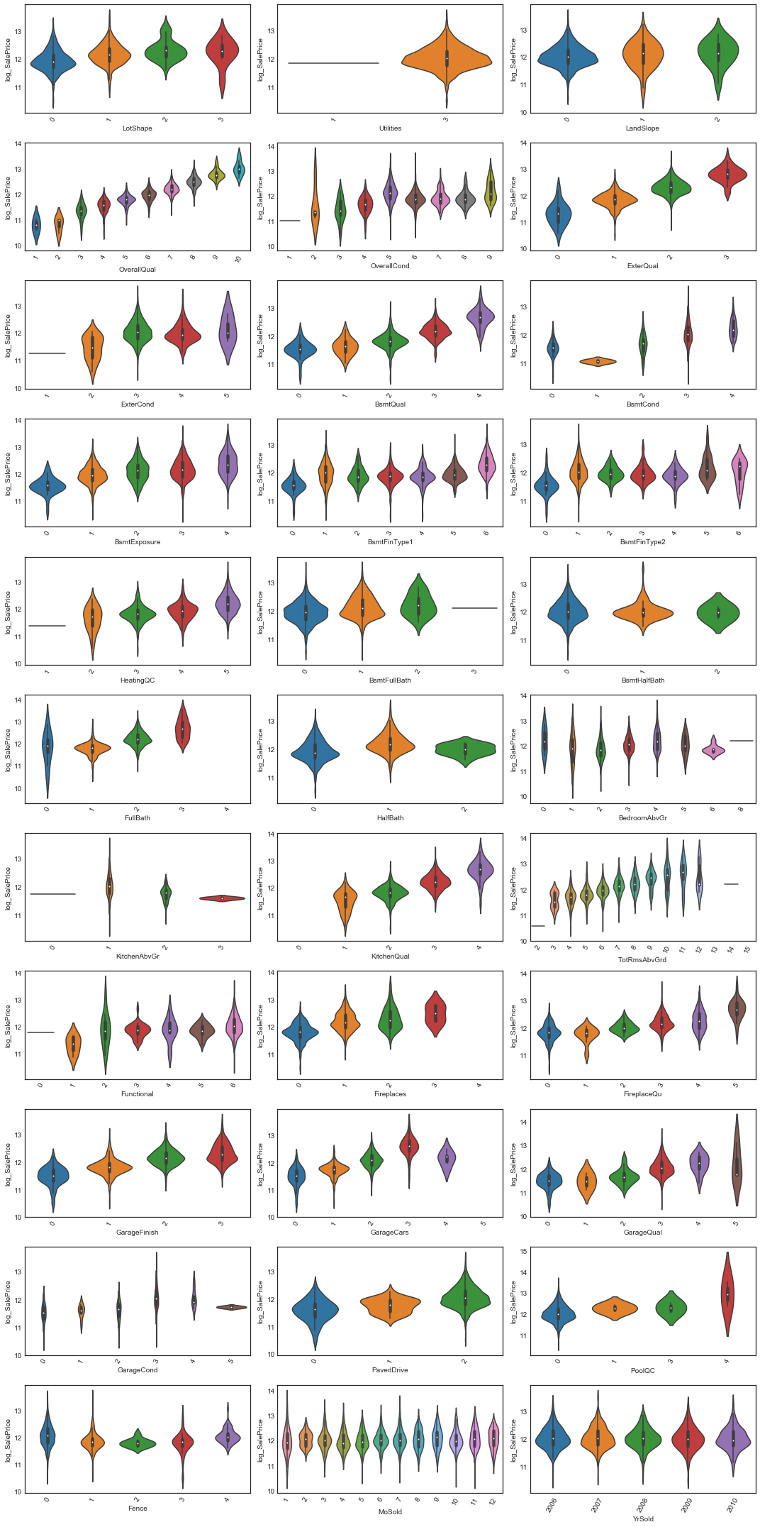
# plot dependence distance with log_SalePrice
D_dep_response(ords.data, 'log_SalePrice').sort_values(by='D').T
| MoSold | OverallQual | TotRmsAbvGrd | BsmtFinType1 | YrSold | GarageCars | BsmtQual | GarageFinish | FireplaceQu | OverallCond | ... | GarageQual | ExterCond | GarageCond | PavedDrive | Functional | BsmtHalfBath | LandSlope | KitchenAbvGr | PoolQC | Utilities | |
|---|---|---|---|---|---|---|---|---|---|---|---|---|---|---|---|---|---|---|---|---|---|
| D | 0.795577 | 0.821511 | 0.83499 | 0.859118 | 0.877148 | 0.879704 | 0.879858 | 0.886311 | 0.886812 | 0.890191 | ... | 0.951855 | 0.957094 | 0.959353 | 0.962894 | 0.965643 | 0.978447 | 0.979514 | 0.981345 | 0.997317 | 0.999801 |
1 rows × 33 columns
Again variables with unbalanced distributions (e.g. PoolQc, Utilities) tend to have high dependence distance, as do variables for which the distribution of log_SalePrice doesn’t differ much across their classes (e.g. BsmtHalfBath, PavedDrive, LandSlope).
That OverallQual has high dependence with SalePrice isn’t surprising, but perhaps MoSold having the lowest is.
Rank correlation hypothesis tests
One way of testing statistical dependence between ordered varialbes is using rank correlations. Since they’re relatively straightforward to calculate, we calculate three common ones and compare. We’ll look at Pearson’s , Spearman’s , and Kendall’s
# rank correlation results as dataframes
rho_df = rank_hyp_test(ords, 'rho', ss.pearsonr)
r_s_df = rank_hyp_test(ords, 'r_s', ss.spearmanr)
tau_df = rank_hyp_test(ords, 'tau', ss.kendalltau)
rank_hyp_test_dfs = {'rho': rho_df, 'r_s': r_s_df, 'tau': tau_df}

# rank and sort by p-value of Pearson's rho
get_rank_corr_df(rank_hyp_test_dfs).drop(columns=['rho', 'r_s', 'tau']).sort_values(by='rho_p_val_rank')
| rho_p_val | rho_p_val_rank | r_s_p_val | r_s_p_val_rank | tau_p_val | tau_p_val_rank | |
|---|---|---|---|---|---|---|
| OverallQual | 0.000000e+00 | 1 | 0.000000e+00 | 1 | 5.929359e-270 | 1 |
| ExterQual | 7.761033e-201 | 2 | 2.040959e-203 | 3 | 1.272156e-159 | 4 |
| GarageCars | 3.307683e-199 | 3 | 2.382463e-207 | 2 | 6.327182e-176 | 2 |
| KitchenQual | 2.324509e-190 | 4 | 3.122308e-193 | 5 | 1.456887e-158 | 5 |
| BsmtQual | 5.427313e-175 | 5 | 2.488211e-197 | 4 | 1.250445e-164 | 3 |
| GarageFinish | 2.620057e-146 | 6 | 9.382754e-165 | 7 | 2.217914e-140 | 6 |
| FullBath | 1.759447e-141 | 7 | 3.253667e-167 | 6 | 1.117470e-133 | 7 |
| FireplaceQu | 3.528296e-114 | 8 | 7.777438e-110 | 8 | 1.384314e-99 | 9 |
| TotRmsAbvGrd | 3.524836e-110 | 9 | 4.199477e-108 | 9 | 5.527766e-104 | 8 |
| Fireplaces | 2.049485e-89 | 10 | 2.189811e-101 | 10 | 5.443444e-88 | 10 |
| HeatingQC | 2.503143e-82 | 11 | 2.833473e-89 | 11 | 5.700439e-81 | 11 |
| GarageQual | 1.143613e-46 | 12 | 1.501771e-43 | 13 | 2.160589e-41 | 13 |
| BsmtExposure | 3.598521e-45 | 13 | 1.337016e-41 | 15 | 1.843618e-40 | 14 |
| GarageCond | 5.806508e-45 | 14 | 1.512574e-40 | 16 | 2.197488e-38 | 16 |
| BsmtFinType1 | 1.544276e-39 | 15 | 2.791158e-46 | 12 | 2.122343e-46 | 12 |
| HalfBath | 6.573728e-35 | 16 | 9.576207e-42 | 14 | 3.530858e-39 | 15 |
| PavedDrive | 1.174245e-32 | 17 | 9.055822e-28 | 18 | 6.292790e-27 | 18 |
| LotShape | 3.682206e-29 | 18 | 3.397766e-36 | 17 | 1.363538e-34 | 17 |
| BsmtCond | 1.302478e-26 | 19 | 1.100259e-25 | 19 | 4.811484e-25 | 19 |
| BsmtFullBath | 5.765714e-20 | 20 | 4.174597e-18 | 21 | 1.040257e-17 | 21 |
| BedroomAbvGr | 5.553622e-16 | 21 | 6.069682e-20 | 20 | 2.027010e-20 | 20 |
| KitchenAbvGr | 1.568173e-08 | 22 | 2.543739e-10 | 23 | 3.235206e-10 | 23 |
| Functional | 1.437417e-07 | 23 | 9.116464e-08 | 24 | 9.253383e-08 | 24 |
| Fence | 2.386137e-05 | 24 | 4.477501e-13 | 22 | 1.551382e-12 | 22 |
| PoolQC | 1.030024e-03 | 25 | 1.490013e-02 | 27 | 1.492559e-02 | 27 |
| MoSold | 2.677357e-02 | 26 | 7.253421e-03 | 26 | 6.503260e-03 | 26 |
| ExterCond | 5.869885e-02 | 27 | 6.460164e-01 | 32 | 6.635896e-01 | 33 |
| YrSold | 1.550808e-01 | 28 | 2.543787e-01 | 30 | 2.573829e-01 | 30 |
| OverallCond | 1.567476e-01 | 29 | 6.717184e-07 | 25 | 1.787177e-07 | 25 |
| LandSlope | 1.671482e-01 | 30 | 7.277014e-02 | 28 | 7.323031e-02 | 28 |
| BsmtFinType2 | 5.861356e-01 | 31 | 1.246273e-01 | 29 | 1.412702e-01 | 29 |
| Utilities | 6.304159e-01 | 32 | 5.249597e-01 | 31 | 5.247749e-01 | 31 |
| BsmtHalfBath | 8.503143e-01 | 33 | 6.522158e-01 | 33 | 6.520497e-01 | 32 |
There is more or less good agreement of -value rankings among the rank correlation hypothesis tests. In particular for a 95% significance level all three fail to reject the null for MoSold, ExterCond, OverallCond, LandSlope, BsmtFinType2, Utilities and BsmtHalfBath. Applying a stricter value of 99.9% significance, all three reject PoolQC as well.
It’s important to recognize that rank correlation tests are measures of monotonicity (the tendency of variables to increase together and decrease together). They may fail to detect non-linear relationships that are not monotonic. In our particular case, MoSold had the highest statistical dependence with log_SalePrice among ordinal variables, but all three rank correlation tests reject a relationship between the two at 95% significance.
Quantitative variables
Finally we’ll consider the quantitative variables, that is the continuous variables. In our cleaned dataframe these are the variables with float64 dtype.
# dataframe of quantitative variables
quants = HPDataFramePlus(data=clean.data.select_dtypes('float64').drop(columns=['SalePrice']))
quants.data.head()
| LotFrontage | LotArea | YearBuilt | YearRemodAdd | MasVnrArea | BsmtFinSF1 | BsmtFinSF2 | BsmtUnfSF | TotalBsmtSF | 1stFlrSF | ... | GrLivArea | GarageYrBlt | GarageArea | WoodDeckSF | OpenPorchSF | EnclosedPorch | 3SsnPorch | ScreenPorch | PoolArea | MiscVal | ||
|---|---|---|---|---|---|---|---|---|---|---|---|---|---|---|---|---|---|---|---|---|---|---|
| Id | ||||||||||||||||||||||
| train | 1 | 65.0 | 8450.0 | 2003.0 | 2003.0 | 196.0 | 706.0 | 0.0 | 150.0 | 856.0 | 856.0 | ... | 1710.0 | 2003.0 | 548.0 | 0.0 | 61.0 | 0.0 | 0.0 | 0.0 | 0.0 | 0.0 |
| 2 | 80.0 | 9600.0 | 1976.0 | 1976.0 | 0.0 | 978.0 | 0.0 | 284.0 | 1262.0 | 1262.0 | ... | 1262.0 | 1976.0 | 460.0 | 298.0 | 0.0 | 0.0 | 0.0 | 0.0 | 0.0 | 0.0 | |
| 3 | 68.0 | 11250.0 | 2001.0 | 2002.0 | 162.0 | 486.0 | 0.0 | 434.0 | 920.0 | 920.0 | ... | 1786.0 | 2001.0 | 608.0 | 0.0 | 42.0 | 0.0 | 0.0 | 0.0 | 0.0 | 0.0 | |
| 4 | 60.0 | 9550.0 | 1915.0 | 1970.0 | 0.0 | 216.0 | 0.0 | 540.0 | 756.0 | 961.0 | ... | 1717.0 | 1998.0 | 642.0 | 0.0 | 35.0 | 272.0 | 0.0 | 0.0 | 0.0 | 0.0 | |
| 5 | 84.0 | 14260.0 | 2000.0 | 2000.0 | 350.0 | 655.0 | 0.0 | 490.0 | 1145.0 | 1145.0 | ... | 2198.0 | 2000.0 | 836.0 | 192.0 | 84.0 | 0.0 | 0.0 | 0.0 | 0.0 | 0.0 |
5 rows × 22 columns
quants.data.info()
<class 'pandas.core.frame.DataFrame'>
MultiIndex: 2916 entries, (train, 1) to (test, 2919)
Data columns (total 22 columns):
LotFrontage      2916 non-null float64
LotArea          2916 non-null float64
YearBuilt        2916 non-null float64
YearRemodAdd     2916 non-null float64
MasVnrArea       2916 non-null float64
BsmtFinSF1       2916 non-null float64
BsmtFinSF2       2916 non-null float64
BsmtUnfSF        2916 non-null float64
TotalBsmtSF      2916 non-null float64
1stFlrSF         2916 non-null float64
2ndFlrSF         2916 non-null float64
LowQualFinSF     2916 non-null float64
GrLivArea        2916 non-null float64
GarageYrBlt      2916 non-null float64
GarageArea       2916 non-null float64
WoodDeckSF       2916 non-null float64
OpenPorchSF      2916 non-null float64
EnclosedPorch    2916 non-null float64
3SsnPorch        2916 non-null float64
ScreenPorch      2916 non-null float64
PoolArea         2916 non-null float64
MiscVal          2916 non-null float64
dtypes: float64(22)
memory usage: 532.7+ KB
# print description of quantitative variables
quants.desc = desc
quants.print_desc(cols=quants.data.columns)
LotFrontage: Linear feet of street connected to property


LotArea: Lot size in square feet


YearBuilt: Original construction date


YearRemodAdd: Remodel date (same as construction date if no remodeling or additions)


MasVnrArea: Masonry veneer area in square feet


BsmtFinSF1: Type 1 finished square feet


BsmtFinSF2: Type 2 finished square feet


BsmtUnfSF: Unfinished square feet of basement area


TotalBsmtSF: Total square feet of basement area


1stFlrSF: First Floor square feet


2ndFlrSF: Second floor square feet


LowQualFinSF: Low quality finished square feet (all floors)


GrLivArea: Above grade (ground) living area square feet


GarageYrBlt: Year garage was built


GarageArea: Size of garage in square feet


WoodDeckSF: Wood deck area in square feet


OpenPorchSF: Open porch area in square feet


EnclosedPorch: Enclosed porch area in square feet


3SsnPorch: Three season porch area in square feet


ScreenPorch: Screen porch area in square feet


PoolArea: Pool area in square feet


MiscVal: $Value of miscellaneous feature
quants.data.info()
<class 'pandas.core.frame.DataFrame'>
MultiIndex: 2916 entries, (train, 1) to (test, 2919)
Data columns (total 22 columns):
LotFrontage      2916 non-null float64
LotArea          2916 non-null float64
YearBuilt        2916 non-null float64
YearRemodAdd     2916 non-null float64
MasVnrArea       2916 non-null float64
BsmtFinSF1       2916 non-null float64
BsmtFinSF2       2916 non-null float64
BsmtUnfSF        2916 non-null float64
TotalBsmtSF      2916 non-null float64
1stFlrSF         2916 non-null float64
2ndFlrSF         2916 non-null float64
LowQualFinSF     2916 non-null float64
GrLivArea        2916 non-null float64
GarageYrBlt      2916 non-null float64
GarageArea       2916 non-null float64
WoodDeckSF       2916 non-null float64
OpenPorchSF      2916 non-null float64
EnclosedPorch    2916 non-null float64
3SsnPorch        2916 non-null float64
ScreenPorch      2916 non-null float64
PoolArea         2916 non-null float64
MiscVal          2916 non-null float64
dtypes: float64(22)
memory usage: 532.7+ KB
# plot distributions of quantitative variables
plot_cont_dists(nrows=6, ncols=4, data=quants.data, figsize=(15, 20))
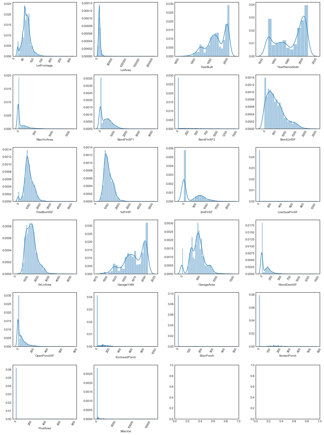
Most of the variables are highly positively skewed
quants.data.skew()
LotFrontage       1.049465
LotArea          13.269377
YearBuilt        -0.600024
YearRemodAdd     -0.449893
MasVnrArea        2.618990
BsmtFinSF1        0.982465
BsmtFinSF2        4.145816
BsmtUnfSF         0.919998
TotalBsmtSF       0.677494
1stFlrSF          1.259407
2ndFlrSF          0.861482
LowQualFinSF     12.088646
GrLivArea         1.069506
GarageYrBlt      -0.658118
GarageArea        0.219101
WoodDeckSF        1.847119
OpenPorchSF       2.533111
EnclosedPorch     4.003630
3SsnPorch        11.375940
ScreenPorch       3.946335
PoolArea         17.694707
MiscVal          21.947201
dtype: float64
Some of the quantitative variables appear to be multimodal. For quite a few, this is due to a large peak at zero, and for some it’s clear that zero is being used as a stand-in for a null value (for example, PoolArea = 0 if the house has no pool). We’ll look at which variables have a high peak at zero
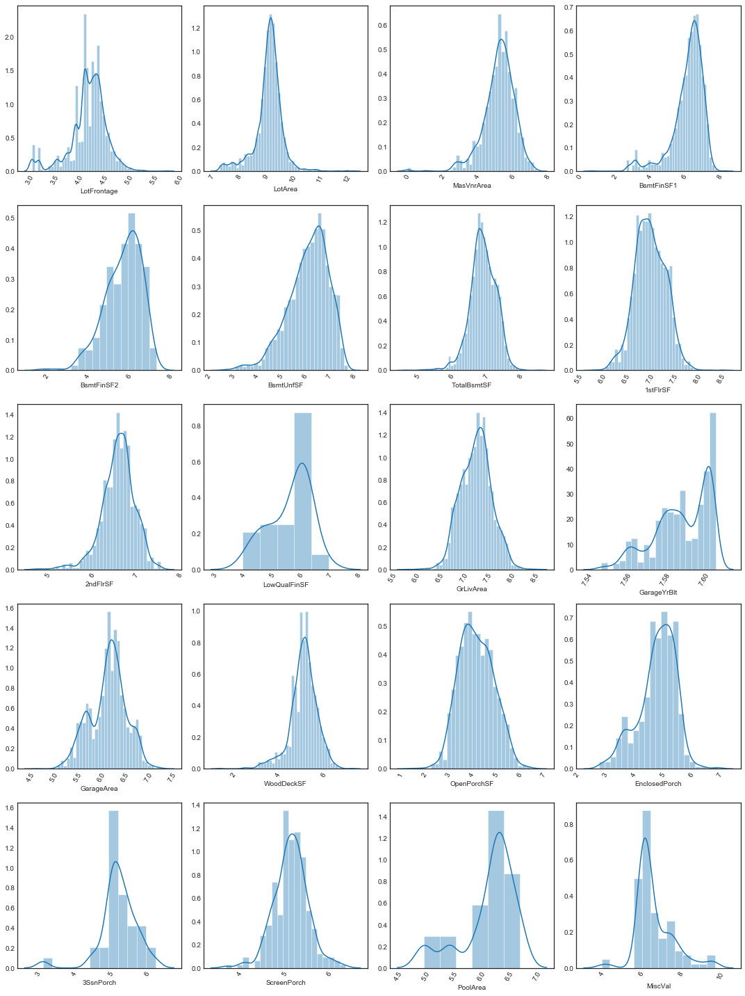
We note that many of these variables have long right tails, so logarithmic scales may be more appropriate for these.
# plot distributions of logarithms of all nonzero values of quantitative variables
log_cols = quants.data.columns.drop(['YearBuilt', 'YearRemodAdd'])
plot_log_cont_dists(nrows=5, ncols=4, data=quants.data, log_cols=log_cols, figsize=(15, 20))
Relationships among quantitative variables
# scatterplots of quantitative variables
sns.pairplot(quants.data)
<seaborn.axisgrid.PairGrid at 0x121036da0>
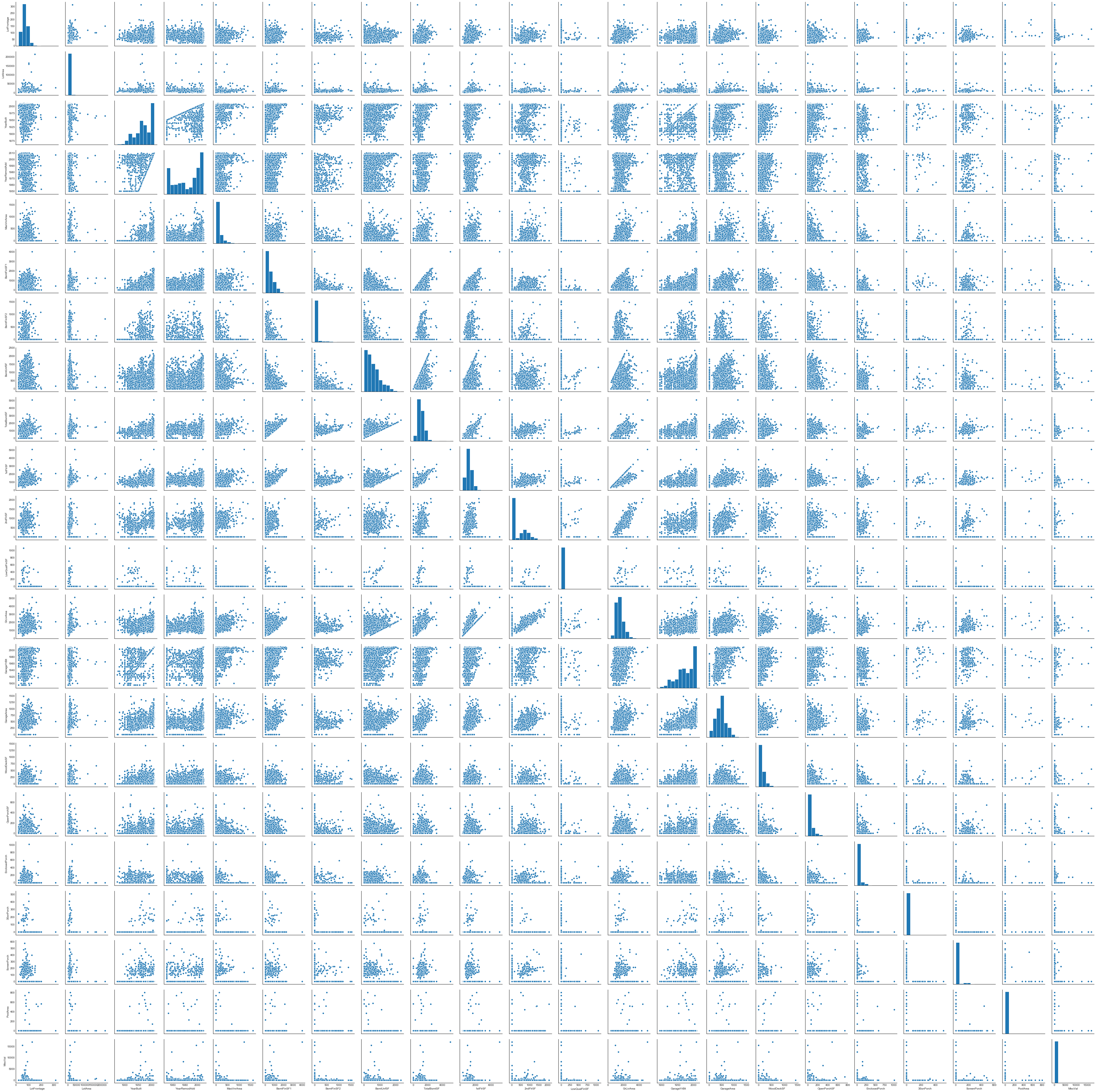
While pairplots can be helpful, this one is a bit too big to be of much use, although it may inform later methods of detecting relationships.
Some things do stand out:
-
There appear to be regions of exclusion for certain pairs of variables, probably due to impossible values. For example,
YrRemodAddis never greater thanYrBuilt. -
Many of the distributions are very concentrated.
LotArea,BsmtFinSF2,LowQualFinSF,EnclosedPorch,3SsnPorchall stand out as extremely concentrated.
Now we’ll look at dependencies among the quantitative variables
# dataframe of dependence distances of quantitative variables
quants_D_dep_df = D_dep(quants.data)
# plot dependence distance
plot_D_dep(D_dep_df=quants_D_dep_df, figsize=(15, 10))
# plot lower dependence distances of quantitative variables
plot_low_D_dep(D_dep_df=quants_D_dep_df, D_threshold=0.8, figsize=(13, 8))
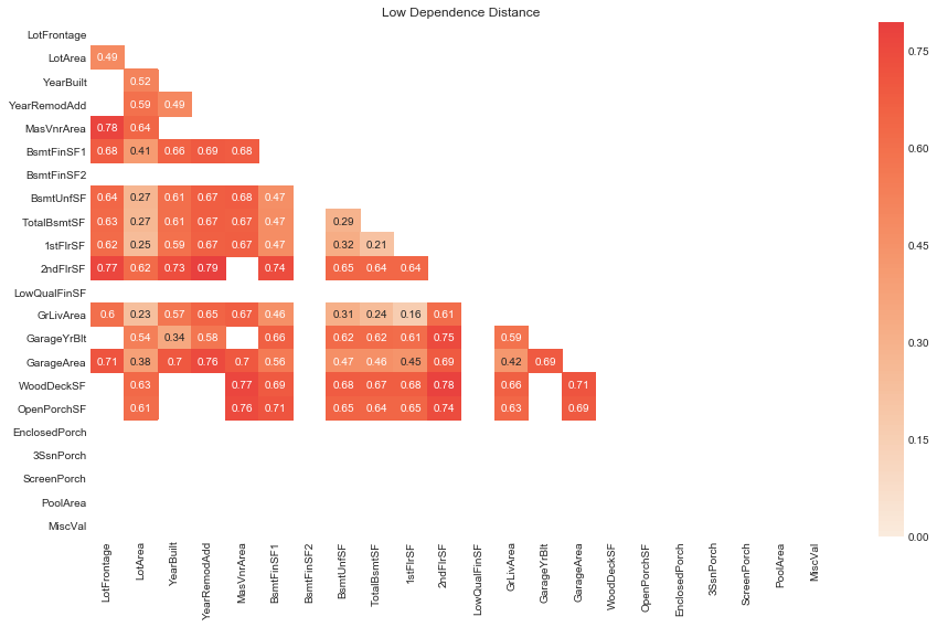
# display pairs of quantitatives with low dependence distance
rank_pairs_by_D(D_dep_df=quants_D_dep_df, D_threshold=0.8).head(10)
| var1 | var2 | D | |
|---|---|---|---|
| 1 | 1stFlrSF | GrLivArea | 0.158882 |
| 2 | TotalBsmtSF | 1stFlrSF | 0.213738 |
| 3 | LotArea | GrLivArea | 0.227010 |
| 4 | TotalBsmtSF | GrLivArea | 0.242833 |
| 5 | LotArea | 1stFlrSF | 0.250292 |
| 6 | LotArea | TotalBsmtSF | 0.269834 |
| 7 | LotArea | BsmtUnfSF | 0.273087 |
| 8 | BsmtUnfSF | TotalBsmtSF | 0.292260 |
| 9 | BsmtUnfSF | GrLivArea | 0.307987 |
| 10 | BsmtUnfSF | 1stFlrSF | 0.320845 |
Compared to quantitative and ordinal variables pairs, pairs of quantitative variables are showing much higher dependencies (lower dependence distances) overall. For many of these pairs , the high dependence makes sense given both variables are measuring very similar areas, for example, 1stFlrSF, GrLivArea and TotalBsmtSF.
We expect that Pearsons’ (i.e. correlation/linear dependence) of these variables should be high as well.
# plot pearson's correlation for quantitative variables
plot_corr(quants_data=quants.data, figsize=(15, 10))
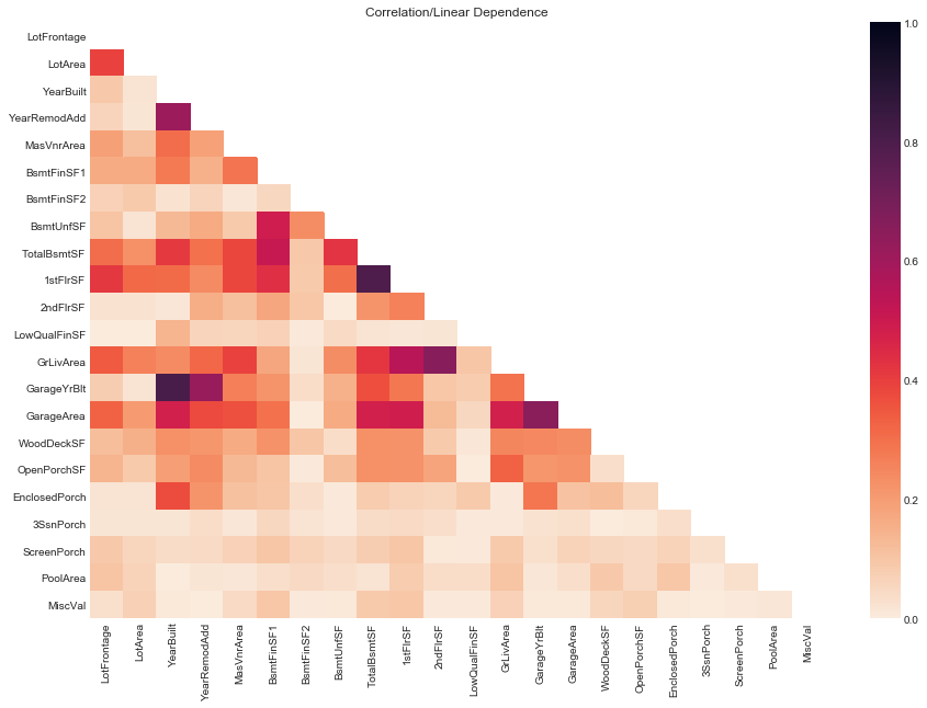
# plot high absolute value of correlations of quantiatives
plot_high_corr(quants_data=quants.data, abs_corr_threshold=0.5, figsize=(15, 10))
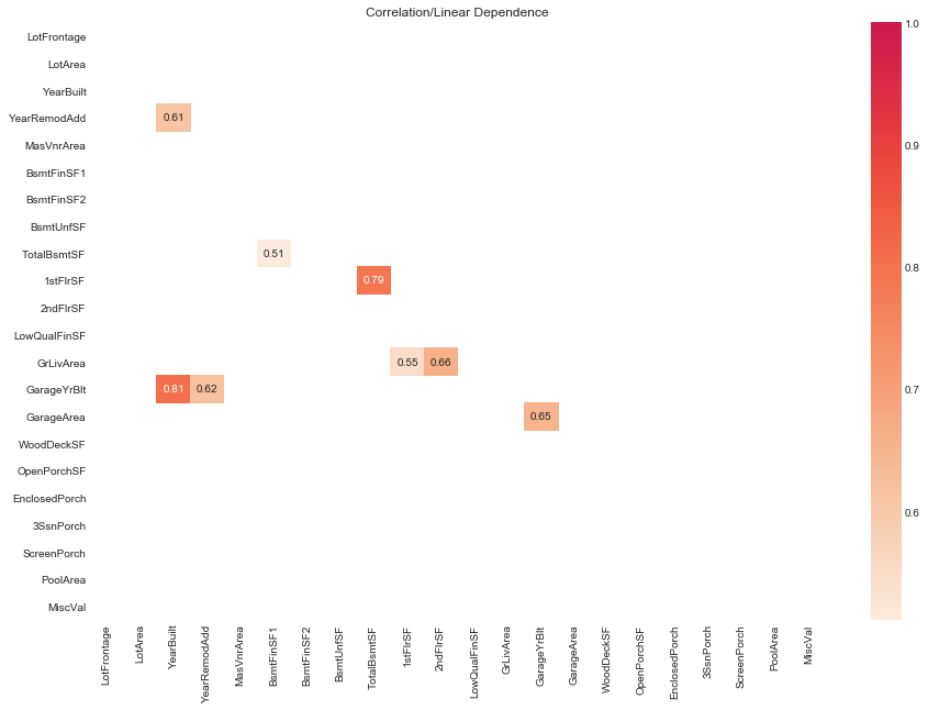
# rank pairs of quantitatives by absolute values of correlation
rank_pairs_by_abs_corr_df = rank_pairs_by_abs_corr(quants_data=quants.data, abs_corr_threshold=0.5)
rank_pairs_by_abs_corr_df
| var1 | var2 | abs_corr | |
|---|---|---|---|
| 1 | BsmtFinSF1 | TotalBsmtSF | 0.511258 |
| 2 | 1stFlrSF | GrLivArea | 0.546383 |
| 3 | YearBuilt | YearRemodAdd | 0.612023 |
| 4 | YearRemodAdd | GarageYrBlt | 0.618881 |
| 5 | GarageYrBlt | GarageArea | 0.653440 |
| 6 | 2ndFlrSF | GrLivArea | 0.658420 |
| 7 | TotalBsmtSF | 1stFlrSF | 0.793482 |
| 8 | YearBuilt | GarageYrBlt | 0.808100 |
Relationships between quantitatives and SalePrice
# add log_SalePrice to quantitatives dataframe
quants.data['log_SalePrice'] = np.log(clean.data['SalePrice'])
quants.data['log_SalePrice']
       Id
train  1       12.247694
       2       12.109011
       3       12.317167
       4       11.849398
       5       12.429216
                 ...
test   2915          NaN
       2916          NaN
       2917          NaN
       2918          NaN
       2919          NaN
Name: log_SalePrice, Length: 2916, dtype: float64
# plot joint distributions of quantitative variables and log of sale price
plot_joint_dists_with_response(nrows=6, ncols=4, quants_data=quants.data, response='log_SalePrice', figsize=(15, 20))
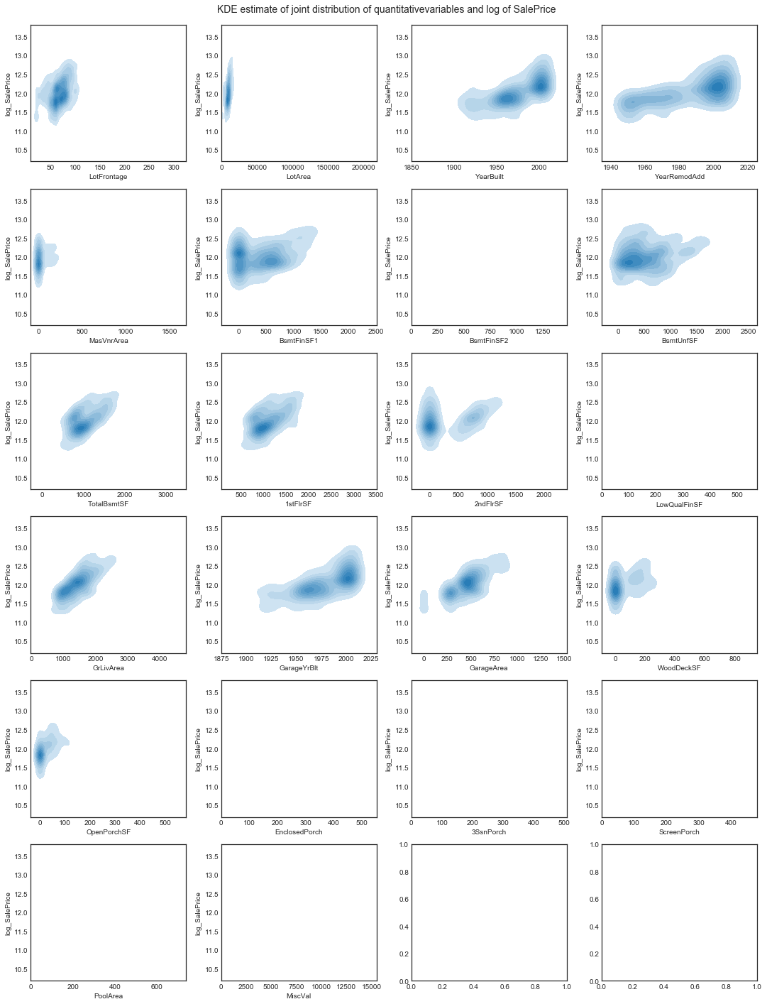
The distribution of some of the variables appears to be problematic for seaborn to fit a joint kernel density estimate. We’ll look at scatterplots instead
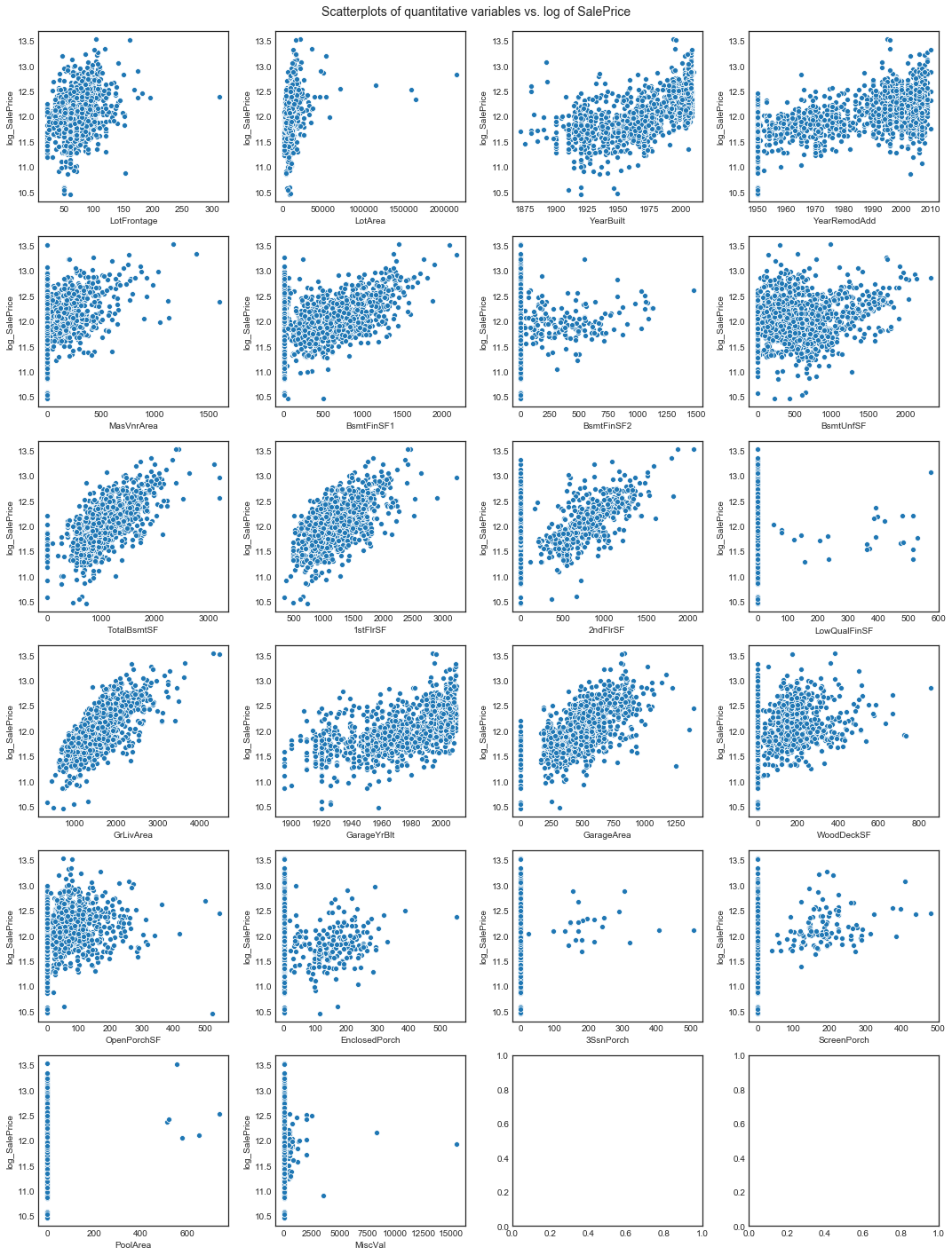
# scatterplots of quantitative variables and log of sale price
plot_scatter_with_response(nrows=6, ncols=4, quants_data=quants.data, response='log_SalePrice', figsize=(15, 20))
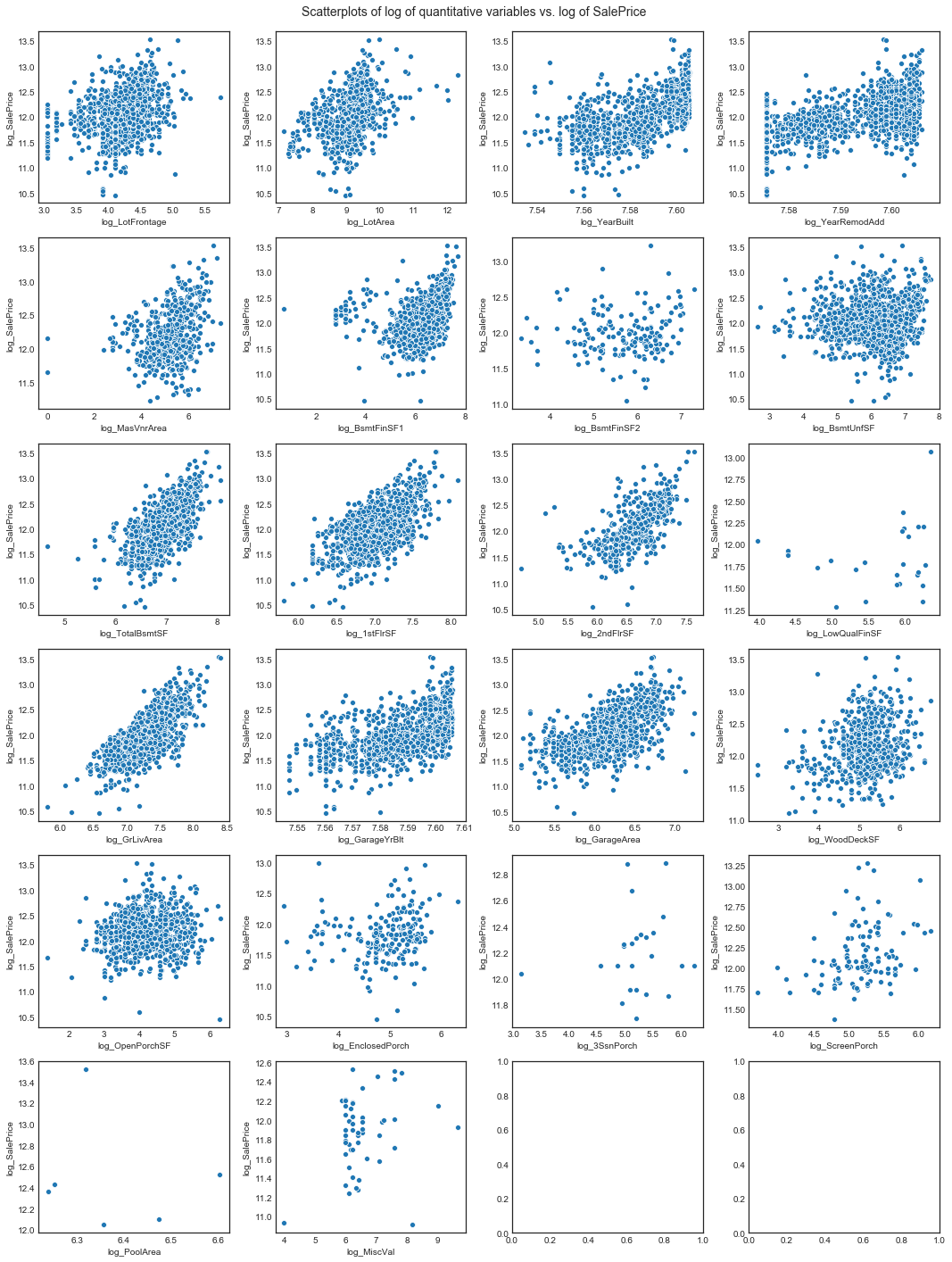
Now will look at scatterplots of log transformations of the quantitive variables vs. log_SalePrice
# scatterplots of log of nonzero values of quantitative variables and log of sale price
plot_log_scatter_with_response(nrows=6, ncols=4, quants_data=quants.data, response='log_SalePrice', figsize=(15, 20))
# rank dependence distance of quantiatives with log_SalePrice
D_dep_response(data=quants.data, response='log_SalePrice').sort_values(by='D').T
| LotArea | GrLivArea | 1stFlrSF | BsmtUnfSF | TotalBsmtSF | GarageArea | BsmtFinSF1 | YearBuilt | GarageYrBlt | LotFrontage | ... | YearRemodAdd | WoodDeckSF | MasVnrArea | EnclosedPorch | BsmtFinSF2 | ScreenPorch | MiscVal | LowQualFinSF | 3SsnPorch | PoolArea | |
|---|---|---|---|---|---|---|---|---|---|---|---|---|---|---|---|---|---|---|---|---|---|
| D | 0.166598 | 0.216601 | 0.243486 | 0.259179 | 0.266558 | 0.390699 | 0.41101 | 0.549621 | 0.561122 | 0.579528 | ... | 0.627967 | 0.632256 | 0.647403 | 0.854684 | 0.875006 | 0.913641 | 0.968622 | 0.985514 | 0.98756 | 0.995242 |
1 rows × 22 columns
Considering the scatterplots and taking into account the dependence distance , we see that some quantitative variables appear likely to be less helpful in predicting SalePrice. Of these, EnclosedPorch, BsmtFinSF2, ScreenPorch, MiscVal, LowQualFinSF, 3SSnPorch, and PoolArea stand out (all have )