Explore Fashion MNIST dataset and CNN model

Here we’ll get a feel for the Fashion MNIST image data and the model we’ll be using to classify those images.

Later we’ll train, tune and test the model

Setup
The Fashion MNIST image data set
- Class representative images
- Class distributions
Keras CNN model for classification
- Overview
- Train default model locally

Setup

%matplotlib inline
import matplotlib.pyplot as plt
import numpy as np
import pandas as pd
import os


# filter out FutureWarnings
from warnings import simplefilter
simplefilter(action='ignore', category=FutureWarning)

# Supress Tensorflow Warnings
import tensorflow.compat.v1.logging as logging
logging.set_verbosity(logging.ERROR)

# custom model class
from cnn import FashionMNISTCNN

Using TensorFlow backend.

The Fashion MNIST image data set

More information on the dataset see Github or Kaggle. We’ll use the .csv files from Kaggle for data exploration.

train_data, val_data = pd.read_csv('data/train.csv'), pd.read_csv('data/val.csv')

train_data.info()

<class 'pandas.core.frame.DataFrame'>
RangeIndex: 60000 entries, 0 to 59999
Columns: 785 entries, label to pixel784
dtypes: int64(785)
memory usage: 359.3 MB

val_data.info()

<class 'pandas.core.frame.DataFrame'>
RangeIndex: 10000 entries, 0 to 9999
Columns: 785 entries, label to pixel784
dtypes: int64(785)
memory usage: 59.9 MB

There are 60,000 images in the training set, and 10,000 in the validation set.
There are 785 features - a class label and 784 pixels. A row of 784 pixels is a flattened 28 x 28 pixel array

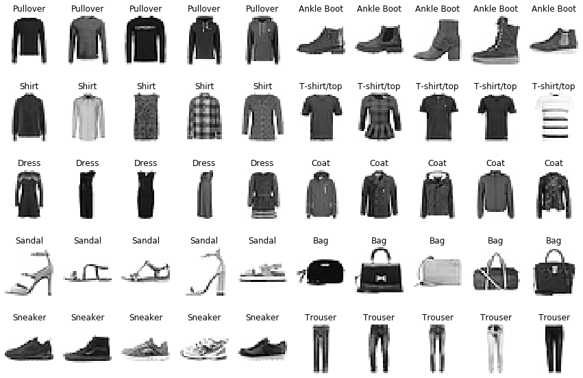
Class representative images

There are 10 image classes

def add_class_str_labels(df):
    class_str_labels = ["T-shirt/top", "Trouser", "Pullover", "Dress", "Coat", "Sandal", 
                "Shirt", "Sneaker", "Bag", "Ankle Boot"]
    # dict for mapping labels to string labels
    class_mapping = {i: label for (i, label) in enumerate(class_str_labels)}
    df['str_label'] = df['label'].apply(lambda x: class_str_labels[x])
    
add_class_str_labels(train_data)
add_class_str_labels(val_data)

We’ll collect 5 images from each of the 10 classes and plot them

def get_class_images(df, class_str_label, num_images=5):
    # slice all rows for this class
    class_slice = df[df['str_label'] == class_str_label]
    # get 5 random indices
    indices = np.random.choice(class_slice.index.values, size=5, replace=False)
    # slice images for these indices
    image_slice = class_slice.loc[indices, : ]
    # return array of 28 x 28 images
    return image_slice.drop(columns=['label', 'str_label']).values.reshape(5, 28, 28)

def plot_sample_images(df):
    class_str_labels=df['str_label'].unique()
    fig, ax = plt.subplots(5, 10, figsize=(15, 10))
    for (i, label) in enumerate(class_str_labels):
        class_images = get_class_images(df, label)
        for (j, image) in enumerate(class_images):
            ax[i//2, j + 5*(i%2)].imshow(image, cmap='Greys')
            ax[i//2, j + 5*(i%2)].axis('off')
            ax[i//2, j + 5*(i%2)].set_title(label)
            
plot_sample_images(train_data)

png

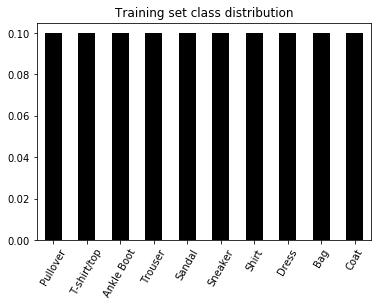
Class distributions

We’ll look at how the images are distributed across the image classes in the train and validation sets

# plot class distributions for training and validation data
def plot_class_distribution(df, title):
    class_dist = train_data['str_label'].value_counts() / len(train_data)
    class_dist.plot(kind='bar', color='k')
    plt.title(title)
    plt.xticks(rotation=60)

plot_class_distribution(train_data, 'Training set class distribution')

png

plot_class_distribution(val_data, 'Validation set class distribution')

png

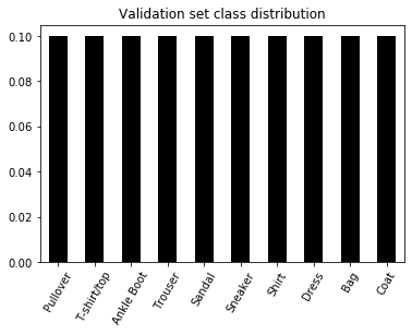
The classes are perfectly balanced.

Before we begin training a model, we’ll create a perfectly balanced test set from the training data

def balanced_test_split(df, size=10000):
    np.random.seed(27)
    df = df.copy()
    # get class names
    class_str_labels = df['str_label'].unique()
    # store slices for later concatenation
    slices = []
    # get slices for all the classes
    for class_str_label in class_str_labels:
        # slice all rows for this class
        class_slice = df[df['str_label'] == class_str_label]
        # get indices for test rows
        indices = np.random.choice(class_slice.index.values, 
                                             size=size//10, 
                                             replace=False)
        # slice for these indices
        slices += [class_slice.loc[indices, : ]]
        # drop rows for these indices 
        df = df.drop(index=indices)
    # collect slices into a dataframe
    test_df = pd.concat(slices, ignore_index=True)
    return df, test_df

train_data, test_data = balanced_test_split(train_data)

train_data.info()

<class 'pandas.core.frame.DataFrame'>
Int64Index: 50000 entries, 0 to 59999
Columns: 786 entries, label to str_label
dtypes: int64(785), object(1)
memory usage: 300.2+ MB

test_data.info()

<class 'pandas.core.frame.DataFrame'>
RangeIndex: 10000 entries, 0 to 9999
Columns: 786 entries, label to str_label
dtypes: int64(785), object(1)
memory usage: 60.0+ MB

Keras CNN Model for classification

Overview

The model we’ll use is a convolutional neural network build using Keras with Tensorflow backend. The CNN is implemented as a wrapper for the Keras functional API class keras.models.Model

The model architecture follows the convention of several convolutional/pooling blocks, then a flattening, followed by a few fully connected layers and finally a softmax layer.

Convolutional/Pooling blocks - Each convolutional block follows the sequence:
1. Zero padding
2. 2D convolution
3. Batch Normalization
4. Activation
5. 2D Max Pooling
Fully Connected layers - Each fully connected layer follows the sequence:
1. Batch Normalization
2. Dropout
3. Activation

INPUT_SHAPE = (28, 28, 1)
model = FashionMNISTCNN(INPUT_SHAPE)

The FashionMNISTCNN class constructor accepts a dictionary of architecture parameters which constructs an arbitary number of conv/pool blocks followed by an arbitarary number of fully connected layers.

By default the CNN has 3 conv/pool layers, 2 fully connected layers, and a softmax layer.

# Default parameters for convolutional/pooling blocks
model.conv_params

{'conv0': {'conv0_pad': 1,
  'conv0_channels': 32,
  'conv0_filter': 3,
  'conv0_stride': 1,
  'conv0_pool': 1,
  'conv0_activation': 'relu'},
 'conv1': {'conv1_pad': 1,
  'conv1_channels': 64,
  'conv1_filter': 3,
  'conv1_stride': 1,
  'conv1_pool': 2,
  'conv1_activation': 'relu'},
 'conv2': {'conv2_pad': 1,
  'conv2_channels': 128,
  'conv2_filter': 3,
  'conv2_stride': 1,
  'conv2_pool': 2,
  'conv2_activation': 'relu'}}

# Default parameters for fully connected layers
model.fc_params

{'fc0': {'fc0_neurons': 512, 'fc0_activation': 'relu'},
 'fc1': {'fc1_neurons': 256, 'fc1_activation': 'relu'},
 'fc2': {'fc2_neurons': 10, 'fc2_activation': 'softmax'}}

We’ll inspect the default model with keras built in summary

model.summary()

Model: "fashionmnistcnn_1"
_________________________________________________________________
Layer (type)                 Output Shape              Param #   
=================================================================
input_1 (InputLayer)         (None, 28, 28, 1)         0         
_________________________________________________________________
conv0_pad (ZeroPadding2D)    (None, 30, 30, 1)         0         
_________________________________________________________________
conv0 (Conv2D)               (None, 28, 28, 32)        320       
_________________________________________________________________
conv0_bn (BatchNormalization (None, 28, 28, 32)        128       
_________________________________________________________________
conv0_act (Activation)       (None, 28, 28, 32)        0         
_________________________________________________________________
conv0_pool (MaxPooling2D)    (None, 28, 28, 32)        0         
_________________________________________________________________
conv1_pad (ZeroPadding2D)    (None, 30, 30, 32)        0         
_________________________________________________________________
conv1 (Conv2D)               (None, 28, 28, 64)        18496     
_________________________________________________________________
conv1_bn (BatchNormalization (None, 28, 28, 64)        256       
_________________________________________________________________
conv1_act (Activation)       (None, 28, 28, 64)        0         
_________________________________________________________________
conv1_pool (MaxPooling2D)    (None, 14, 14, 64)        0         
_________________________________________________________________
conv2_pad (ZeroPadding2D)    (None, 16, 16, 64)        0         
_________________________________________________________________
conv2 (Conv2D)               (None, 14, 14, 128)       73856     
_________________________________________________________________
conv2_bn (BatchNormalization (None, 14, 14, 128)       512       
_________________________________________________________________
conv2_act (Activation)       (None, 14, 14, 128)       0         
_________________________________________________________________
conv2_pool (MaxPooling2D)    (None, 7, 7, 128)         0         
_________________________________________________________________
flatten_1 (Flatten)          (None, 6272)              0         
_________________________________________________________________
fc0_bn (BatchNormalization)  (None, 6272)              25088     
_________________________________________________________________
fc0_drop (Dropout)           (None, 6272)              0         
_________________________________________________________________
fc0_act (Dense)              (None, 512)               3211776   
_________________________________________________________________
fc1_bn (BatchNormalization)  (None, 512)               2048      
_________________________________________________________________
fc1_drop (Dropout)           (None, 512)               0         
_________________________________________________________________
fc1_act (Dense)              (None, 256)               131328    
_________________________________________________________________
fc2_bn (BatchNormalization)  (None, 256)               1024      
_________________________________________________________________
fc2_drop (Dropout)           (None, 256)               0         
_________________________________________________________________
fc2_act (Dense)              (None, 10)                2570      
=================================================================
Total params: 3,467,402
Trainable params: 3,452,874
Non-trainable params: 14,528
_________________________________________________________________

Train default model locally

We’ll train the model for a few epochs locally to get a rough sense of how it’s going to go

# prepare data for model fitting
X_train, Y_train, X_val, Y_val, X_test, Y_test = model.load_data()
X_train, Y_train, X_val, Y_val, X_test, Y_test = model.prepare_data(X_train, Y_train, X_val, Y_val, X_test, Y_test)

# train model for a few epochs with no dropout
model.compile()
history = model.fit(X_train, Y_train, X_val, Y_val, epochs=5, batch_size=50)

Train on 50000 samples, validate on 10000 samples
Epoch 1/1
50000/50000 [==============================] - 640s 13ms/step - loss: 0.3524 - acc: 0.8742 - val_loss: 0.3688 - val_acc: 0.8599

Epoch 00001: val_acc improved from -inf to 0.85990, saving model to models/keras_checkpoints/FashionMNISTCNN-epoch-01-val_acc-0.8599.hdf5
best_val_acc: 0.8598999953269959

Keras CNN for Fashion MNIST Image classification