islr notes and exercises from An Introduction to Statistical Learning
10. Unsupervised Learning
Exercise 9: Hierarchical Clustering on USArrests dataset
Preparing the data
Information on the dataset can be found here
%matplotlib inline
import matplotlib.pyplot as plt
import pandas as pd
import numpy as np
import seaborn as sns; sns.set_style('whitegrid')
arrests = pd.read_csv('../../datasets/USAressts.csv', index_col=0)
arrests.head()
| Murder | Assault | UrbanPop | Rape | |
|---|---|---|---|---|
| Alabama | 13.2 | 236 | 58 | 21.2 |
| Alaska | 10.0 | 263 | 48 | 44.5 |
| Arizona | 8.1 | 294 | 80 | 31.0 |
| Arkansas | 8.8 | 190 | 50 | 19.5 |
| California | 9.0 | 276 | 91 | 40.6 |
arrests.info()
<class 'pandas.core.frame.DataFrame'>
Index: 50 entries, Alabama to Wyoming
Data columns (total 4 columns):
Murder      50 non-null float64
Assault     50 non-null int64
UrbanPop    50 non-null int64
Rape        50 non-null float64
dtypes: float64(2), int64(2)
memory usage: 2.0+ KB
a. Cluster with complete linkage and Euclidean distance
from scipy.cluster.hierarchy import dendrogram, linkage

Z = linkage(arrests, method='complete', metric='Euclidean')

plt.figure(figsize=(10, 8))
plt.title('Complete Linkage Dendrogram')
plt.xlabel('sample')
plt.ylabel('Euclidean Distance')
d_1 = dendrogram(Z, labels=arrests.index, leaf_rotation=90)
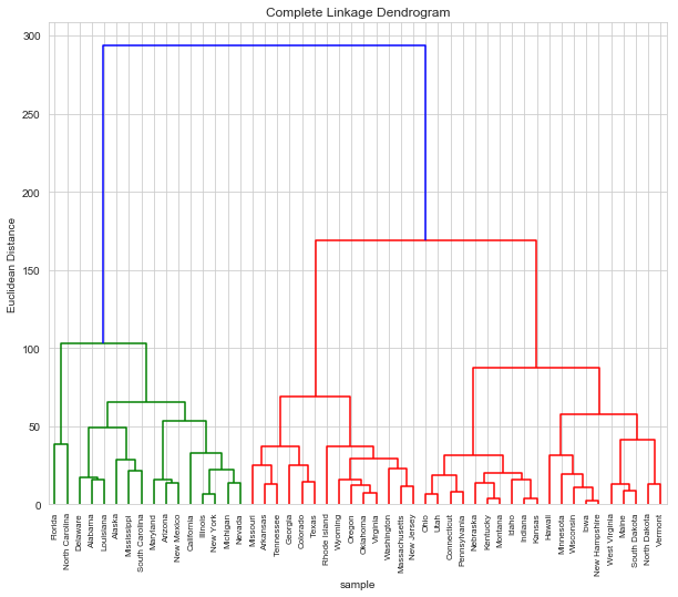
b. Cut dendrogram to get 3 clusters
The clusters are
cluster_1 = d_1['ivl'][:d_1['ivl'].index('Nevada') + 1]
cluster_1
['Florida',
 'North Carolina',
 'Delaware',
 'Alabama',
 'Louisiana',
 'Alaska',
 'Mississippi',
 'South Carolina',
 'Maryland',
 'Arizona',
 'New Mexico',
 'California',
 'Illinois',
 'New York',
 'Michigan',
 'Nevada']
cluster_2 = d_!['ivl'][d_1['ivl'].index('Nevada') + 1: d_1['ivl'].index('New Jersey') + 1]
cluster_2
['Missouri',
 'Arkansas',
 'Tennessee',
 'Georgia',
 'Colorado',
 'Texas',
 'Rhode Island',
 'Wyoming',
 'Oregon',
 'Oklahoma',
 'Virginia',
 'Washington',
 'Massachusetts',
 'New Jersey']
cluster_3 = d_1['ivl'][d_1['ivl'].index('New Jersey') + 1 :]
cluster_3
['Ohio',
 'Utah',
 'Connecticut',
 'Pennsylvania',
 'Nebraska',
 'Kentucky',
 'Montana',
 'Idaho',
 'Indiana',
 'Kansas',
 'Hawaii',
 'Minnesota',
 'Wisconsin',
 'Iowa',
 'New Hampshire',
 'West Virginia',
 'Maine',
 'South Dakota',
 'North Dakota',
 'Vermont']
c. Repeat clustering after scaling
arrests_sc = arrests/arrests.std()

Z = linkage(arrests_sc, method='complete', metric='Euclidean')

plt.figure(figsize=(10, 8))
plt.title('Complete Linkage Dendrogram')
plt.xlabel('sample')
plt.ylabel('Euclidean Distance')
d_2 = dendrogram(Z, labels=arrests_sc.index, leaf_rotation=90)
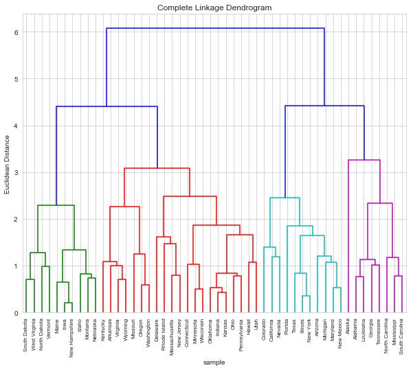
d. What effect does scaling have?
Scaling seemingly results in a more “balanced” clustering. In general we know that data should be scaled if variables are measured on incomparable scales (see conceptual exercise 5 for an example). In this case, while Murder, Assault and Rape are measured in the same units, Urban is measured in a percentage.
Thus we conclude the data should be scaled bofore clustering in this case.