islr notes and exercises from An Introduction to Statistical Learning
9. Support Vector Machines
Exercise 7: Using SVMs to classify mileage in Auto dataset
%matplotlib inline
import matplotlib.pyplot as plt
import matplotlib.pyplot as plt
import numpy as np
import pandas as pd
import seaborn as sns; sns.set_style('whitegrid')
import warnings
warnings.simplefilter(action='ignore', category=FutureWarning)
Preparing the data
auto = pd.read_csv('../../datasets/Auto.csv', index_col=0)
auto.reset_index(inplace=True, drop=True)
auto.head()
| mpg | cylinders | displacement | horsepower | weight | acceleration | year | origin | name | |
|---|---|---|---|---|---|---|---|---|---|
| 0 | 18.0 | 8 | 307.0 | 130 | 3504 | 12.0 | 70 | 1 | chevrolet chevelle malibu |
| 1 | 15.0 | 8 | 350.0 | 165 | 3693 | 11.5 | 70 | 1 | buick skylark 320 |
| 2 | 18.0 | 8 | 318.0 | 150 | 3436 | 11.0 | 70 | 1 | plymouth satellite |
| 3 | 16.0 | 8 | 304.0 | 150 | 3433 | 12.0 | 70 | 1 | amc rebel sst |
| 4 | 17.0 | 8 | 302.0 | 140 | 3449 | 10.5 | 70 | 1 | ford torino |
auto.info()
<class 'pandas.core.frame.DataFrame'>
RangeIndex: 392 entries, 0 to 391
Data columns (total 9 columns):
mpg             392 non-null float64
cylinders       392 non-null int64
displacement    392 non-null float64
horsepower      392 non-null int64
weight          392 non-null int64
acceleration    392 non-null float64
year            392 non-null int64
origin          392 non-null int64
name            392 non-null object
dtypes: float64(3), int64(5), object(1)
memory usage: 27.6+ KB
a. Create high/low mileage variable and preprocess
# add mileage binary variable
auto['high_mpg'] = (auto['mpg'] > auto['mpg'].median()).astype(int)

auto.head()
| mpg | cylinders | displacement | horsepower | weight | acceleration | year | origin | name | high_mpg | |
|---|---|---|---|---|---|---|---|---|---|---|
| 0 | 18.0 | 8 | 307.0 | 130 | 3504 | 12.0 | 70 | 1 | chevrolet chevelle malibu | 0 |
| 1 | 15.0 | 8 | 350.0 | 165 | 3693 | 11.5 | 70 | 1 | buick skylark 320 | 0 |
| 2 | 18.0 | 8 | 318.0 | 150 | 3436 | 11.0 | 70 | 1 | plymouth satellite | 0 |
| 3 | 16.0 | 8 | 304.0 | 150 | 3433 | 12.0 | 70 | 1 | amc rebel sst | 0 |
| 4 | 17.0 | 8 | 302.0 | 140 | 3449 | 10.5 | 70 | 1 | ford torino | 0 |
We found this article helpful. We’ll scale the data to the interval [0, 1].
df = auto.drop(columns=['name'])
df = (df - df.min())/(df.max() - df.min())
b. Linear SVC
from sklearn.svm import SVC
from sklearn.model_selection import GridSearchCV

# rough tuning param
param = {'C': np.logspace(0, 9, 10)}
linear_svc = SVC(kernel='linear')
linear_svc_search = GridSearchCV(estimator=linear_svc,
                                 param_grid=param,
                                 cv=7,
                                 scoring='accuracy')
X, Y = df.drop(columns=['high_mpg']), auto['high_mpg']
%timeit -n1 -r1 linear_svc_search.fit(X, Y)
804 ms ± 0 ns per loop (mean ± std. dev. of 1 run, 1 loop each)
linear_svc_search_df = pd.DataFrame(linear_svc_search.cv_results_)
linear_svc_search_df[['param_C', 'mean_test_score']]
| param_C | mean_test_score | |
|---|---|---|
| 0 | 1 | 0.908163 |
| 1 | 10 | 0.969388 |
| 2 | 100 | 0.984694 |
| 3 | 1000 | 0.997449 |
| 4 | 10000 | 0.997449 |
| 5 | 100000 | 0.997449 |
| 6 | 1e+06 | 0.997449 |
| 7 | 1e+07 | 0.997449 |
| 8 | 1e+08 | 0.997449 |
| 9 | 1e+09 | 0.997449 |
linear_svc_search.best_params_
{'C': 1000.0}
linear_svc_search.best_score_
0.9974489795918368
# fine tuning param
param = {'C': np.linspace(500, 1500, 1000)}
linear_svc = SVC(kernel='linear')
linear_svc_search = GridSearchCV(estimator=linear_svc,
                                 param_grid=param,
                                 cv=7,
                                 scoring='accuracy')
%timeit -n1 -r1 linear_svc_search.fit(X, Y)
54.5 s ± 0 ns per loop (mean ± std. dev. of 1 run, 1 loop each)
linear_svc_search.best_params_
{'C': 696.1961961961962}
linear_svc_search.best_score_
0.9974489795918368
c. Nonlinear SVCs
Polynomial SVC
# rough param tuning
params = {'C': np.logspace(-4, 4, 9),
          'gamma': np.logspace(-4, 4, 9),
          'degree': [2, 3]}
poly_svc = SVC(kernel='poly')
poly_svc_search = GridSearchCV(estimator=poly_svc,
                                 param_grid=params,
                                 cv=7,
                                 scoring='accuracy')
%timeit -n1 -r1 poly_svc_search.fit(X, Y)
8.7 s ± 0 ns per loop (mean ± std. dev. of 1 run, 1 loop each)
poly_svc_search.best_params_
{'C': 0.001, 'degree': 2, 'gamma': 100.0}
poly_svc_search.best_score_
0.9617346938775511
params = {'C': np.linspace(0.0001, 0.01, 20),
          'gamma': np.linspace(50, 150, 20)}
poly_svc = SVC(kernel='poly', degree=2)
poly_svc_search = GridSearchCV(estimator=poly_svc,
                                 param_grid=params,
                                 cv=7,
                                 scoring='accuracy')
%timeit -n1 -r1 poly_svc_search.fit(X, Y)
19.3 s ± 0 ns per loop (mean ± std. dev. of 1 run, 1 loop each)
poly_svc_search.best_params_
{'C': 0.0068736842105263166, 'gamma': 50.0}
poly_svc_search.best_score_
0.9668367346938775
Radial SVC
# rough param tuning
params = {'C': np.logspace(-4, 4, 9),
          'gamma': np.logspace(-4, 4, 9)}
radial_svc = SVC(kernel='rbf')
radial_svc_search = GridSearchCV(estimator=radial_svc,
                                 param_grid=params,
                                 cv=7,
                                 scoring='accuracy')
%timeit -n1 -r1 radial_svc_search.fit(X, Y)
5.34 s ± 0 ns per loop (mean ± std. dev. of 1 run, 1 loop each)
radial_svc_search.best_params_
{'C': 1000.0, 'gamma': 0.01}
radial_svc_search.best_score_
0.9795918367346939
params = {'C': np.logspace(4, 9, 5),
          'gamma': np.linspace(0.001, 0.1, 100)}
radial_svc = SVC(kernel='rbf')
radial_svc_search = GridSearchCV(estimator=radial_svc,
                                 param_grid=params,
                                 cv=7,
                                 scoring='accuracy')
%timeit -n1 -r1 radial_svc_search.fit(X, Y)
20.9 s ± 0 ns per loop (mean ± std. dev. of 1 run, 1 loop each)
radial_svc_search.best_params_
{'C': 177827.94100389228, 'gamma': 0.002}
radial_svc_search.best_score_
0.9974489795918368
d. CV error plots
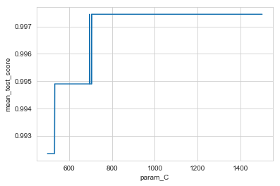
Linear SVC
linear_svc_df = pd.DataFrame(linear_svc_search.cv_results_)
sns.lineplot(x=linear_svc_df['param_C'], y=linear_svc_df['mean_test_score'])
<matplotlib.axes._subplots.AxesSubplot at 0x1a1f5e42b0>
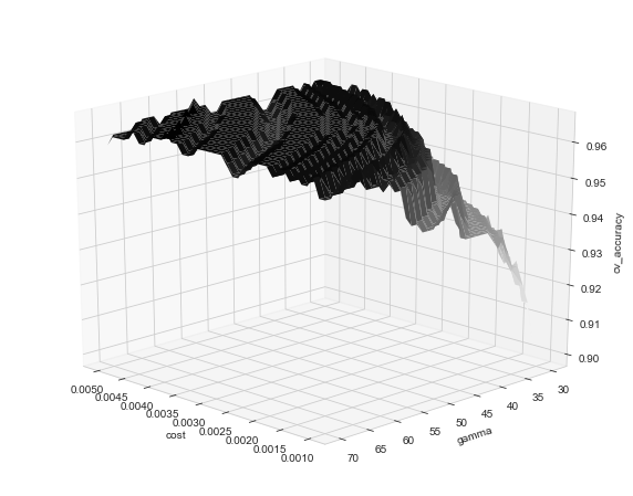
Quadratic SVC
from mpl_toolkits import mplot3d

poly_svc_df = pd.DataFrame(poly_svc_search.cv_results_)

cost, gamma = poly_svc_df['param_C'].unique(), poly_svc_df['param_gamma'].unique()

X, Y = np.meshgrid(cost, gamma)
Z = scores = poly_svc_df['mean_test_score'].values.reshape(len(cost), len(gamma))

fig = plt.figure(figsize=(10, 8))
ax = plt.axes(projection='3d')
ax.plot_surface(X, Y, Z, rstride=1, cstride=1,
                cmap='Greys', edgecolor='none')
ax.set_xlabel('cost')
ax.set_ylabel('gamma')
ax.set_zlabel('cv_accuracy');
ax.view_init(20, 135)
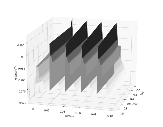
radial_svc_df = pd.DataFrame(radial_svc_search.cv_results_)

cost, gamma = radial_svc_df['param_C'].unique(), radial_svc_df['param_gamma'].unique()

X, Y = np.meshgrid(cost, gamma)
Z = scores = radial_svc_df['mean_test_score'].values.reshape(len(gamma), len(cost))

fig = plt.figure(figsize=(10, 8))
ax = plt.axes(projection='3d')
ax.plot_surface(X, Y, Z, rstride=1, cstride=1,
                cmap='Greys', edgecolor='none')
ax.set_xlabel('cost')
ax.set_ylabel('gamma')
ax.set_zlabel('cv_accuracy');
ax.view_init(20, 15)