islr notes and exercises from An Introduction to Statistical Learning
9. Support Vector Machines
Exercise 4: Comparing polynomial, radial, and linear kernel SVMs on a simulated dataset
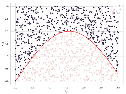
Generating the data
%matplotlib inline
import matplotlib.pyplot as plt
import numpy as np
import pandas as pd
import seaborn as sns; sns.set_style('whitegrid')
import warnings
warnings.simplefilter(action='ignore', category=FutureWarning)
X = np.random.uniform(0, 3, size=(1000, 2))
Y = np.array([1 if X[i, 1] > 2 * np.sin(X[i, 0]) else -1 for i in range(X.shape[0])])
data = pd.DataFrame({'X_1': X[:, 0], 'X_2': X[:, 1], 'Y': Y})
plt.figure(figsize=(8, 6))
sns.scatterplot(x=data['X_1'], y=data['X_2'], data=data, hue='Y')
x = np.linspace(0, 3, 50)
plt.plot(x, 2* np.sin(x), 'r')
[<matplotlib.lines.Line2D at 0x1a1dc46eb8>]
Train test split
from sklearn.model_selection import train_test_split

X, Y = data[['X_1', 'X_2']], data['Y']

X_train, X_test, y_train, y_test = train_test_split(X, Y, train_size=100)
SVMs with linear, polynomial, and radial kernels
Note that what the authors call the support vector classifier is the support vector machine with linear kernel.
Fit models
from sklearn.svm import SVC
from sklearn.metrics import accuracy_score

svc_linear = SVC(kernel='linear')
svc_linear.fit(X_train, y_train)

svc_poly = SVC(kernel='poly', degree=6)
svc_poly.fit(X_train, y_train)

svc_rbf = SVC(kernel='rbf')
svc_rbf.fit(X_train, y_train)
SVC(C=1.0, cache_size=200, class_weight=None, coef0=0.0,
  decision_function_shape='ovr', degree=3, gamma='auto_deprecated',
  kernel='rbf', max_iter=-1, probability=False, random_state=None,
  shrinking=True, tol=0.001, verbose=False)
data_train = pd.concat([X_train, y_train], axis=1)
data_train['linear_pred'] = svc_linear.predict(X_train)
data_train['poly_pred'] = svc_poly.predict(X_train)
data_train['rbf_pred'] = svc_rbf.predict(X_train)
data_train.head()
| X_1 | X_2 | Y | linear_pred | poly_pred | rbf_pred | |
|---|---|---|---|---|---|---|
| 105 | 0.358341 | 2.459384 | 1 | 1 | 1 | 1 |
| 446 | 2.103954 | 0.025083 | -1 | -1 | -1 | -1 |
| 232 | 2.035364 | 2.543201 | 1 | 1 | 1 | 1 |
| 559 | 1.507827 | 0.750842 | -1 | -1 | -1 | -1 |
| 418 | 2.756047 | 2.396298 | 1 | 1 | 1 | 1 |
data_test = pd.concat([X_test, y_test], axis=1)
data_test['linear_pred'] = svc_linear.predict(X_test)
data_test['poly_pred'] = svc_poly.predict(X_test)
data_test['rbf_pred'] = svc_rbf.predict(X_test)
data_test.head()
| X_1 | X_2 | Y | linear_pred | poly_pred | rbf_pred | |
|---|---|---|---|---|---|---|
| 127 | 0.490400 | 0.268376 | -1 | -1 | -1 | -1 |
| 837 | 1.329158 | 1.556672 | -1 | 1 | -1 | -1 |
| 518 | 0.769138 | 2.898040 | 1 | 1 | 1 | 1 |
| 743 | 0.678482 | 1.677742 | 1 | 1 | 1 | 1 |
| 61 | 0.375443 | 1.528661 | 1 | 1 | 1 | 1 |
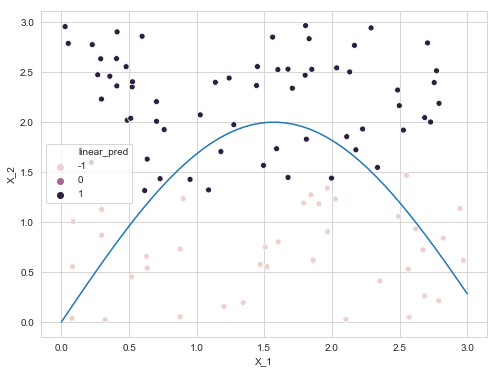
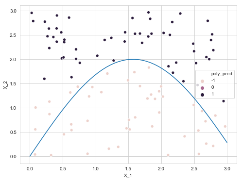
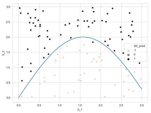
Compare models on the test data
Plot model predictions
plt.figure(figsize=(8, 6))
sns.scatterplot(x='X_1', y='X_2', data=data_train, hue='linear_pred')
x = np.linspace(0, 3, 50)
sns.lineplot(x, 2*np.sin(x))
<matplotlib.axes._subplots.AxesSubplot at 0x1a1b73a9e8>
plt.figure(figsize=(8, 6))
sns.scatterplot(x='X_1', y='X_2', data=data_train, hue='poly_pred')
x = np.linspace(0, 3, 50)
sns.lineplot(x, 2*np.sin(x))
<matplotlib.axes._subplots.AxesSubplot at 0x1a1e8b9630>
plt.figure(figsize=(8, 6))
sns.scatterplot(x='X_1', y='X_2', data=data_train, hue='rbf_pred')
x = np.linspace(0, 3, 50)
sns.lineplot(x, 2*np.sin(x))
<matplotlib.axes._subplots.AxesSubplot at 0x1a1e9289b0>
Train and test errors
from sklearn.metrics import accuracy_score

errors = pd.DataFrame(columns=['train', 'test'], index=['linear', 'poly', 'rbf'])

for model in ['linear', 'poly', 'rbf']:
    errors.at[model, 'train'] = accuracy_score(data_train['Y'], data_train[model+'_pred'])
    errors.at[model, 'test'] = accuracy_score(data_test['Y'], data_test[model+'_pred'])
errors.sort_values('train', ascending=False)
| train | test | |
|---|---|---|
| rbf | 0.97 | 0.965556 |
| poly | 0.92 | 0.908889 |
| linear | 0.84 | 0.838889 |
On both training and testing data, the rankings were the same (1) rbf, (2) degree 2 polynomial, (3) linear.