islr notes and exercises from An Introduction to Statistical Learning
8. Tree-based Methods
Exercise 9: Using tree based methods on the OJ dataset
Preparing the data
Information on the dataset can be found here
%matplotlib inline
import matplotlib.pyplot as plt
import numpy as np
import pandas as pd
import seaborn as sns; sns.set_style('whitegrid')
oj = pd.read_csv('../../datasets/OJ.csv', index_col=0)
oj = oj.reset_index(drop=True)
oj.head()
| Purchase | WeekofPurchase | StoreID | PriceCH | PriceMM | DiscCH | DiscMM | SpecialCH | SpecialMM | LoyalCH | SalePriceMM | SalePriceCH | PriceDiff | Store7 | PctDiscMM | PctDiscCH | ListPriceDiff | STORE | |
|---|---|---|---|---|---|---|---|---|---|---|---|---|---|---|---|---|---|---|
| 0 | CH | 237 | 1 | 1.75 | 1.99 | 0.00 | 0.0 | 0 | 0 | 0.500000 | 1.99 | 1.75 | 0.24 | No | 0.000000 | 0.000000 | 0.24 | 1 |
| 1 | CH | 239 | 1 | 1.75 | 1.99 | 0.00 | 0.3 | 0 | 1 | 0.600000 | 1.69 | 1.75 | -0.06 | No | 0.150754 | 0.000000 | 0.24 | 1 |
| 2 | CH | 245 | 1 | 1.86 | 2.09 | 0.17 | 0.0 | 0 | 0 | 0.680000 | 2.09 | 1.69 | 0.40 | No | 0.000000 | 0.091398 | 0.23 | 1 |
| 3 | MM | 227 | 1 | 1.69 | 1.69 | 0.00 | 0.0 | 0 | 0 | 0.400000 | 1.69 | 1.69 | 0.00 | No | 0.000000 | 0.000000 | 0.00 | 1 |
| 4 | CH | 228 | 7 | 1.69 | 1.69 | 0.00 | 0.0 | 0 | 0 | 0.956535 | 1.69 | 1.69 | 0.00 | Yes | 0.000000 | 0.000000 | 0.00 | 0 |
oj.info()
<class 'pandas.core.frame.DataFrame'>
RangeIndex: 1070 entries, 0 to 1069
Data columns (total 18 columns):
Purchase          1070 non-null object
WeekofPurchase    1070 non-null int64
StoreID           1070 non-null int64
PriceCH           1070 non-null float64
PriceMM           1070 non-null float64
DiscCH            1070 non-null float64
DiscMM            1070 non-null float64
SpecialCH         1070 non-null int64
SpecialMM         1070 non-null int64
LoyalCH           1070 non-null float64
SalePriceMM       1070 non-null float64
SalePriceCH       1070 non-null float64
PriceDiff         1070 non-null float64
Store7            1070 non-null object
PctDiscMM         1070 non-null float64
PctDiscCH         1070 non-null float64
ListPriceDiff     1070 non-null float64
STORE             1070 non-null int64
dtypes: float64(11), int64(5), object(2)
memory usage: 150.5+ KB
# drop superfluous variables
oj = oj.drop(columns=['STORE', 'Store7'])
oj.columns
Index(['Purchase', 'WeekofPurchase', 'StoreID', 'PriceCH', 'PriceMM', 'DiscCH',
       'DiscMM', 'SpecialCH', 'SpecialMM', 'LoyalCH', 'SalePriceMM',
       'SalePriceCH', 'PriceDiff', 'PctDiscMM', 'PctDiscCH', 'ListPriceDiff'],
      dtype='object')
# one hot encode categoricals
cat_vars = ['StoreID', 'Purchase']

oj = pd.get_dummies(data=oj, columns=cat_vars, drop_first=True)
oj.head()
| WeekofPurchase | PriceCH | PriceMM | DiscCH | DiscMM | SpecialCH | SpecialMM | LoyalCH | SalePriceMM | SalePriceCH | PriceDiff | PctDiscMM | PctDiscCH | ListPriceDiff | StoreID_2 | StoreID_3 | StoreID_4 | StoreID_7 | Purchase_MM | |
|---|---|---|---|---|---|---|---|---|---|---|---|---|---|---|---|---|---|---|---|
| 0 | 237 | 1.75 | 1.99 | 0.00 | 0.0 | 0 | 0 | 0.500000 | 1.99 | 1.75 | 0.24 | 0.000000 | 0.000000 | 0.24 | 0 | 0 | 0 | 0 | 0 |
| 1 | 239 | 1.75 | 1.99 | 0.00 | 0.3 | 0 | 1 | 0.600000 | 1.69 | 1.75 | -0.06 | 0.150754 | 0.000000 | 0.24 | 0 | 0 | 0 | 0 | 0 |
| 2 | 245 | 1.86 | 2.09 | 0.17 | 0.0 | 0 | 0 | 0.680000 | 2.09 | 1.69 | 0.40 | 0.000000 | 0.091398 | 0.23 | 0 | 0 | 0 | 0 | 0 |
| 3 | 227 | 1.69 | 1.69 | 0.00 | 0.0 | 0 | 0 | 0.400000 | 1.69 | 1.69 | 0.00 | 0.000000 | 0.000000 | 0.00 | 0 | 0 | 0 | 0 | 1 |
| 4 | 228 | 1.69 | 1.69 | 0.00 | 0.0 | 0 | 0 | 0.956535 | 1.69 | 1.69 | 0.00 | 0.000000 | 0.000000 | 0.00 | 0 | 0 | 0 | 1 | 0 |
oj.info()
<class 'pandas.core.frame.DataFrame'>
RangeIndex: 1070 entries, 0 to 1069
Data columns (total 18 columns):
Purchase          1070 non-null object
WeekofPurchase    1070 non-null int64
StoreID           1070 non-null int64
PriceCH           1070 non-null float64
PriceMM           1070 non-null float64
DiscCH            1070 non-null float64
DiscMM            1070 non-null float64
SpecialCH         1070 non-null int64
SpecialMM         1070 non-null int64
LoyalCH           1070 non-null float64
SalePriceMM       1070 non-null float64
SalePriceCH       1070 non-null float64
PriceDiff         1070 non-null float64
Store7            1070 non-null object
PctDiscMM         1070 non-null float64
PctDiscCH         1070 non-null float64
ListPriceDiff     1070 non-null float64
STORE             1070 non-null int64
dtypes: float64(11), int64(5), object(2)
memory usage: 150.5+ KB
a. Train-test split
from sklearn.model_selection import train_test_split

X, y = oj.drop(columns=['Purchase_MM']), oj['Purchase_MM']
X_train, X_test, y_train, y_test = train_test_split(X, y, train_size=800, random_state=27)
X_train.shape
(800, 18)
b. Classification Tree for predicting Purchase
from sklearn.tree import DecisionTreeClassifier

clf_tree = DecisionTreeClassifier(random_state=27)
clf_tree.fit(X_train, y_train)
DecisionTreeClassifier(class_weight=None, criterion='gini', max_depth=None,
            max_features=None, max_leaf_nodes=None,
            min_impurity_decrease=0.0, min_impurity_split=None,
            min_samples_leaf=1, min_samples_split=2,
            min_weight_fraction_leaf=0.0, presort=False, random_state=27,
            splitter='best')
# training error rate
clf_tree.score(X_train, y_train)
0.98875
# test error rate
clf_tree.score(X_test, y_test)
0.7777777777777778
The following is lifted straight from the sklearn docs:
estimator = clf_tree
n_nodes = estimator.tree_.node_count
children_left = estimator.tree_.children_left
children_right = estimator.tree_.children_right
feature = estimator.tree_.feature
threshold = estimator.tree_.threshold


# The tree structure can be traversed to compute various properties such
# as the depth of each node and whether or not it is a leaf.
node_depth = np.zeros(shape=n_nodes, dtype=np.int64)
is_leaves = np.zeros(shape=n_nodes, dtype=bool)
stack = [(0, -1)]  # seed is the root node id and its parent depth
while len(stack) > 0:
    node_id, parent_depth = stack.pop()
    node_depth[node_id] = parent_depth + 1

    # If we have a test node
    if (children_left[node_id] != children_right[node_id]):
        stack.append((children_left[node_id], parent_depth + 1))
        stack.append((children_right[node_id], parent_depth + 1))
    else:
        is_leaves[node_id] = True

# number of leaves = number of terminal nodes
np.sum(is_leaves)
165
c. Classification tree feature importances
# feature importances
clf_tree_feat_imp = pd.DataFrame({'feature': X_train.columns,
                            'importance': clf_tree.feature_importances_})
clf_tree_feat_imp.sort_values(by='importance', ascending=False)
| feature | importance | |
|---|---|---|
| 7 | LoyalCH | 0.659534 |
| 0 | WeekofPurchase | 0.098166 |
| 10 | PriceDiff | 0.085502 |
| 13 | ListPriceDiff | 0.026363 |
| 8 | SalePriceMM | 0.024777 |
| 1 | PriceCH | 0.016979 |
| 14 | StoreID_2 | 0.013228 |
| 5 | SpecialCH | 0.010388 |
| 9 | SalePriceCH | 0.010037 |
| 15 | StoreID_3 | 0.009939 |
| 17 | StoreID_7 | 0.009578 |
| 2 | PriceMM | 0.007906 |
| 12 | PctDiscCH | 0.007804 |
| 16 | StoreID_4 | 0.006839 |
| 6 | SpecialMM | 0.004914 |
| 11 | PctDiscMM | 0.004139 |
| 4 | DiscMM | 0.003906 |
| 3 | DiscCH | 0.000000 |
d. Classification tree plot
from graphviz import Source
from sklearn import tree
from IPython.display import SVG
graph = Source(tree.export_graphviz(clf_tree, out_file=None, filled=True,
                                    feature_names=X.columns))
display(SVG(graph.pipe(format='svg')))

e. Confusion matrix for test data
This Stack Overflow post was helpful
from sklearn.metrics import confusion_matrix

y_act = pd.Series(['Purchase_CH' if entry == 0 else "Purchase_MM" for entry in y_test],
                  name='Actual')
y_pred = pd.Series(['Purchase_CH' if entry == 0 else "Purchase_MM" for entry in clf_tree.predict(X_test)],
                  name='Predicted')
clf_tree_test_conf = pd.crosstab(y_act, y_pred, margins=True)
clf_tree_test_conf
| Predicted | Purchase_CH | Purchase_MM | All |
|---|---|---|---|
| Actual | |||
| Purchase_CH | 136 | 34 | 170 |
| Purchase_MM | 26 | 74 | 100 |
| All | 162 | 108 | 270 |
f. Cross-validation for optimal tree size
from sklearn.model_selection import GridSearchCV

params = {'max_depth': list(range(1, 800)) + [None]}
clf_tree = DecisionTreeClassifier(random_state=27)
clf_tree_search = GridSearchCV(estimator=clf_tree,
                               param_grid=params,
                               cv=8,
                               scoring='accuracy')

%timeit -n1 -r1 clf_tree_search.fit(X_train, y_train)
44.9 s ± 0 ns per loop (mean ± std. dev. of 1 run, 1 loop each)
clf_tree_search.best_params_
{'max_depth': 2}
clf_tree_search.best_score_
0.8075
g. Plot of CV error vs. tree size
clf_tree_search_df = pd.DataFrame(clf_tree_search.cv_results_)
clf_tree_search_df.head()
| mean_fit_time | std_fit_time | mean_score_time | std_score_time | param_max_depth | params | split0_test_score | split1_test_score | split2_test_score | split3_test_score | ... | split0_train_score | split1_train_score | split2_train_score | split3_train_score | split4_train_score | split5_train_score | split6_train_score | split7_train_score | mean_train_score | std_train_score | |
|---|---|---|---|---|---|---|---|---|---|---|---|---|---|---|---|---|---|---|---|---|---|
| 0 | 0.003523 | 0.000421 | 0.001491 | 0.000361 | 1 | {'max_depth': 1} | 0.801980 | 0.841584 | 0.811881 | 0.76 | ... | 0.816881 | 0.811159 | 0.809728 | 0.817143 | 0.817143 | 0.814551 | 0.810271 | 0.803138 | 0.812502 | 0.004591 |
| 1 | 0.002702 | 0.000291 | 0.001097 | 0.000200 | 2 | {'max_depth': 2} | 0.801980 | 0.841584 | 0.811881 | 0.78 | ... | 0.816881 | 0.811159 | 0.816881 | 0.827143 | 0.821429 | 0.818830 | 0.817404 | 0.810271 | 0.817500 | 0.005043 |
| 2 | 0.003065 | 0.000534 | 0.001211 | 0.000264 | 3 | {'max_depth': 3} | 0.811881 | 0.801980 | 0.831683 | 0.73 | ... | 0.826896 | 0.831187 | 0.836910 | 0.851429 | 0.844286 | 0.841655 | 0.841655 | 0.830243 | 0.838032 | 0.007727 |
| 3 | 0.002972 | 0.000107 | 0.000967 | 0.000055 | 4 | {'max_depth': 4} | 0.801980 | 0.811881 | 0.831683 | 0.73 | ... | 0.856938 | 0.841202 | 0.841202 | 0.868571 | 0.847143 | 0.861626 | 0.858773 | 0.844508 | 0.852495 | 0.009673 |
| 4 | 0.003204 | 0.000121 | 0.000971 | 0.000060 | 5 | {'max_depth': 5} | 0.782178 | 0.821782 | 0.801980 | 0.75 | ... | 0.868383 | 0.852647 | 0.856938 | 0.880000 | 0.865714 | 0.873039 | 0.881598 | 0.864479 | 0.867850 | 0.009552 |
5 rows × 27 columns
x, y = clv_tree_search_df['param_max_depth'], clv_tree_search_df['mean_test_score']
plt.plot(x, y)
[<matplotlib.lines.Line2D at 0x1a19ea4908>]
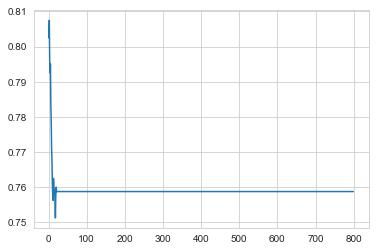
We chose an upper limit of 799 for the maximum tree depth (in a worst case scenario, the decision tree partitions into unique regions for each observation). This is clearly overkill
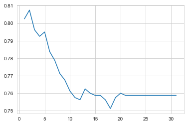
plt.plot(x.loc[:30, ], y.loc[:30, ])
[<matplotlib.lines.Line2D at 0x1a1a67e6d8>]
plt.plot(np.arange(y))
A maximum tree depth of 2 leads to the best cv test error!
i. Pruning a tree with depth 2
from sklearn.model_selection import RandomizedSearchCV

params = {'max_features': np.arange(1, 18),
          'max_leaf_nodes': np.append(np.arange(2, 21), None),
          'min_impurity_decrease': np.linspace(0, 1, 10),
          'min_samples_leaf': np.arange(1, 11)
          }
clf_tree2 = DecisionTreeClassifier(random_state=27, max_depth=2)

# Randomized search to cover a large region of parameter space
clf_tree2_rvsearch = RandomizedSearchCV(estimator=clf_tree2,
                                        param_distributions=params,
                                        cv=8,
                                        scoring='accuracy',
                                        n_iter=1000,
                                        random_state=27)
%timeit -n1 -r1 clf_tree2_rvsearch.fit(X_train, y_train)
39.7 s ± 0 ns per loop (mean ± std. dev. of 1 run, 1 loop each)


/anaconda3/envs/islr/lib/python3.7/site-packages/sklearn/model_selection/_search.py:841: DeprecationWarning: The default of the `iid` parameter will change from True to False in version 0.22 and will be removed in 0.24. This will change numeric results when test-set sizes are unequal.
  DeprecationWarning)
clf_tree2_rvsearch.best_params_
{'min_samples_leaf': 6,
 'min_impurity_decrease': 0.0,
 'max_leaf_nodes': None,
 'max_features': 16}
# Grid search nearby randomized search results
params = {'min_samples_leaf': np.arange(4, 8),
          'max_features': np.arange(10, 16)
         }
clf_tree3 = DecisionTreeClassifier(random_state=27,
                                   max_depth=2,
                                   max_leaf_nodes=None)
clf_tree2_gridsearch = GridSearchCV(estimator=clf_tree3,
                                    param_grid=params,
                                    cv=8,
                                    scoring='accuracy')
%timeit -n1 -r1 clf_tree2_gridsearch.fit(X_train, y_train)
1 s ± 0 ns per loop (mean ± std. dev. of 1 run, 1 loop each)


/anaconda3/envs/islr/lib/python3.7/site-packages/sklearn/model_selection/_search.py:841: DeprecationWarning: The default of the `iid` parameter will change from True to False in version 0.22 and will be removed in 0.24. This will change numeric results when test-set sizes are unequal.
  DeprecationWarning)
clf_tree2_gridsearch.best_params_
{'max_features': 15, 'min_samples_leaf': 4}
clf_tree2_gridsearch.best_score_
0.8075
j. Comparing training error rates
from sklearn.metrics import accuracy_score

# trees for comparison
clf_tree = clf_tree_search.best_estimator_
pruned_clf_tree = clf_tree2_gridsearch.best_estimator_

# train and test errors
train = [accuracy_score(clf_tree.predict(X_train), y_train),
         accuracy_score(pruned_clf_tree.predict(X_train), y_train)]
test = [accuracy_score(clf_tree.predict(X_test), y_test),
         accuracy_score(pruned_clf_tree.predict(X_test), y_test)]

# df for results
comp_df = pd.DataFrame({'train_error': train, 'test_error': test},
                       index=['clf_tree', 'pruned_clf_tree'])
comp_df
| train_error | test_error | |
|---|---|---|
| clf_tree | 0.81625 | 0.785185 |
| pruned_clf_tree | 0.81625 | 0.785185 |