islr notes and exercises from An Introduction to Statistical Learning
8. Tree-based Methods
Conceptual Exercises
- Exercise 1: An example partition/decision tree.
- Exercise 2: Why a boosted stump leads to an additive model
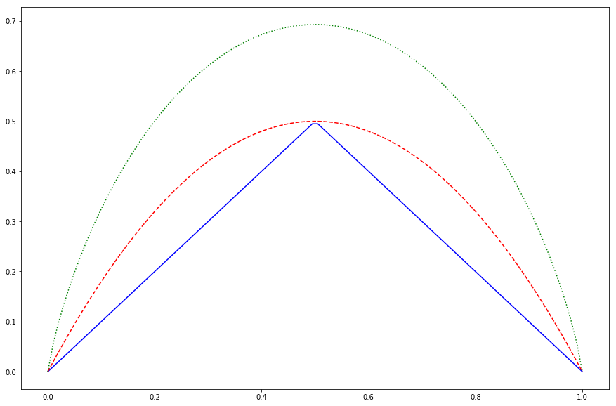
- Exercise 3: Plotting classification error, Gini index, and entropy as functions of for the two class case
- Exercise 4: Sketching trees and partitions
- Exercise 5: Combining bootstrap classification tree predictions
- Exercise 6: A detailed explanation of recursive binary decision tree algorithm for linear regression
Exercise 1: An example partition/decision tree.
Skip.
Exercise 2: Why a boosted stump leads to an additive model
The final form of the boosting model (see algorithm 8.12) is
Since the model is a stump (), for each the estimate is a function of a single predcitor, that is for some . We can then collect terms:
where is a sum over all boosted trees which have as a predictor.
This is the estimate of an additive model.
Exercise 3: Plotting classification error, Gini index, and entropy as functions of for the two class case
%matplotlib inline
import matplotlib.pyplot as plt
import numpy as np

def class_error(p_hat_m1):
    p_hat_m2 = 1 - p_hat_m1
    return 1 - p_hat_m2 if p_hat_m2 >= p_hat_m1 else 1 - p_hat_m1

def gini_index(p_hat_m1):
    p_hat_m2 = 1 - p_hat_m1
    return p_hat_m1 * ( 1 - p_hat_m1) + p_hat_m2 * ( 1 - p_hat_m2)

def entropy(p_hat_m1):
    p_hat_m2 = 1 - p_hat_m1
    if p_hat_m1 in {0, 1}:
        return 0
    else:
        return - np.sum(p_hat_m1 * np.log(p_hat_m1) + p_hat_m2 * np.log(p_hat_m2))

v_class_error = np.vectorize(class_error)
v_gini_index = np.vectorize(gini_index)
v_entropy = np.vectorize(entropy, otypes=[np.float])
x = np.linspace(0, 1, 100)
y_1, y_2, y_3  = v_class_error(x), v_gini_index(x), v_entropy(x)

fig, ax = plt.subplots(figsize=(15, 10))
ax.plot(x, y_1, '-b', label="Classification error")
ax.plot(x, y_2, '--r', label="Gini index")
ax.plot(x, y_3, ':g', label="Entropy")
[<matplotlib.lines.Line2D at 0x11ee4c550>]
Exercise 4: Sketching trees and partitions
Skip
Exercise 5: Combining bootstrap classification tree predictions
The 10 boostrap estimates for are
p_est = np.array([0.1, 0.15, 0.2, 0.2, 0.55, 0.6, 0.6, 0.65, 0.7, 0.75])
p_est
array([0.1 , 0.15, 0.2 , 0.2 , 0.55, 0.6 , 0.6 , 0.65, 0.7 , 0.75])
First we find the classification based on majority vote
# boolean showing if predicted class is red
is_class_red = p_est >= 0.5
# number of times red is predicted
num_red_pred = np.sum(is_class_red)
# predict red if red is the majority vote
if num_red_pred/len(p_est) >= 0.5:
    maj_pred = "Red"
else:
    maj_pred = "Green"

f'majority prediction is {maj_pred}'
'majority prediction is Red'
Next we find the classification based on the average
if np.sum(p_est) >= 0.5:
    avg_pred = "Red"
else:
    avg_pred = "Green"

f'average prediction is {avg_pred}'
'average prediction is Red'
Exercise 6: A detailed explanation of recursive binary decision tree algorithm for linear regression
See our explanation in the notes for § 8.1.1