islr notes and exercises from An Introduction to Statistical Learning
7. Moving Beyond Linearity
Exercise 9: Nonlinear models for predicting nox using dis in Boston dataset
- Preparing the data
- a. Cubic regression
- b. Polynomial regression for degree d = 1, ... ,10
- c. Optimizing the degree of the polynomial regression model
- d. Cubic spline regression with 4 degrees of freedom
- e. Cubic spline regression with degrees of freedom d = 4, ... ,11
- f. Optimizing the degrees of freedom of the cubic spline model
Preparing the data
Information on the dataset can be found here
%matplotlib inline
import matplotlib.pyplot as plt
import numpy as np
import pandas as pd
import seaborn as sns; sns.set_style(style='whitegrid')
boston = pd.read_csv('../../datasets/Boston.csv', index_col=0)
boston = boston.reset_index(drop=True)
boston.head()
| crim | zn | indus | chas | nox | rm | age | dis | rad | tax | ptratio | black | lstat | medv | |
|---|---|---|---|---|---|---|---|---|---|---|---|---|---|---|
| 0 | 0.00632 | 18.0 | 2.31 | 0 | 0.538 | 6.575 | 65.2 | 4.0900 | 1 | 296 | 15.3 | 396.90 | 4.98 | 24.0 |
| 1 | 0.02731 | 0.0 | 7.07 | 0 | 0.469 | 6.421 | 78.9 | 4.9671 | 2 | 242 | 17.8 | 396.90 | 9.14 | 21.6 |
| 2 | 0.02729 | 0.0 | 7.07 | 0 | 0.469 | 7.185 | 61.1 | 4.9671 | 2 | 242 | 17.8 | 392.83 | 4.03 | 34.7 |
| 3 | 0.03237 | 0.0 | 2.18 | 0 | 0.458 | 6.998 | 45.8 | 6.0622 | 3 | 222 | 18.7 | 394.63 | 2.94 | 33.4 |
| 4 | 0.06905 | 0.0 | 2.18 | 0 | 0.458 | 7.147 | 54.2 | 6.0622 | 3 | 222 | 18.7 | 396.90 | 5.33 | 36.2 |
boston.info()
<class 'pandas.core.frame.DataFrame'>
RangeIndex: 506 entries, 0 to 505
Data columns (total 14 columns):
crim       506 non-null float64
zn         506 non-null float64
indus      506 non-null float64
chas       506 non-null int64
nox        506 non-null float64
rm         506 non-null float64
age        506 non-null float64
dis        506 non-null float64
rad        506 non-null int64
tax        506 non-null int64
ptratio    506 non-null float64
black      506 non-null float64
lstat      506 non-null float64
medv       506 non-null float64
dtypes: float64(11), int64(3)
memory usage: 55.4 KB
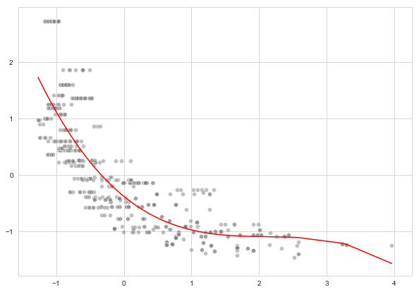
a. Cubic regression
from sklearn.preprocessing import PolynomialFeatures
from sklearn.linear_model import LinearRegression

poly = PolynomialFeatures(degree=3)
linreg = LinearRegression()

X, y = boston['dis'].values, boston['nox'].values
X, y = (X - X.mean())/X.std(), (y - y.mean())/y.std()
linreg.fit(poly.fit_transform(X.reshape(-1, 1)), y)
LinearRegression(copy_X=True, fit_intercept=True, n_jobs=None,
         normalize=False)
import warnings
warnings.simplefilter(action='ignore', category=FutureWarning)
fig = plt.figure(figsize=(10, 7))
sns.lineplot(x=X, y=linreg.predict(poly.fit_transform(X.reshape(-1,1))), color='red')
sns.scatterplot(x=X, y=y, color='grey', alpha=0.5)
<matplotlib.axes._subplots.AxesSubplot at 0x1a2329f320>
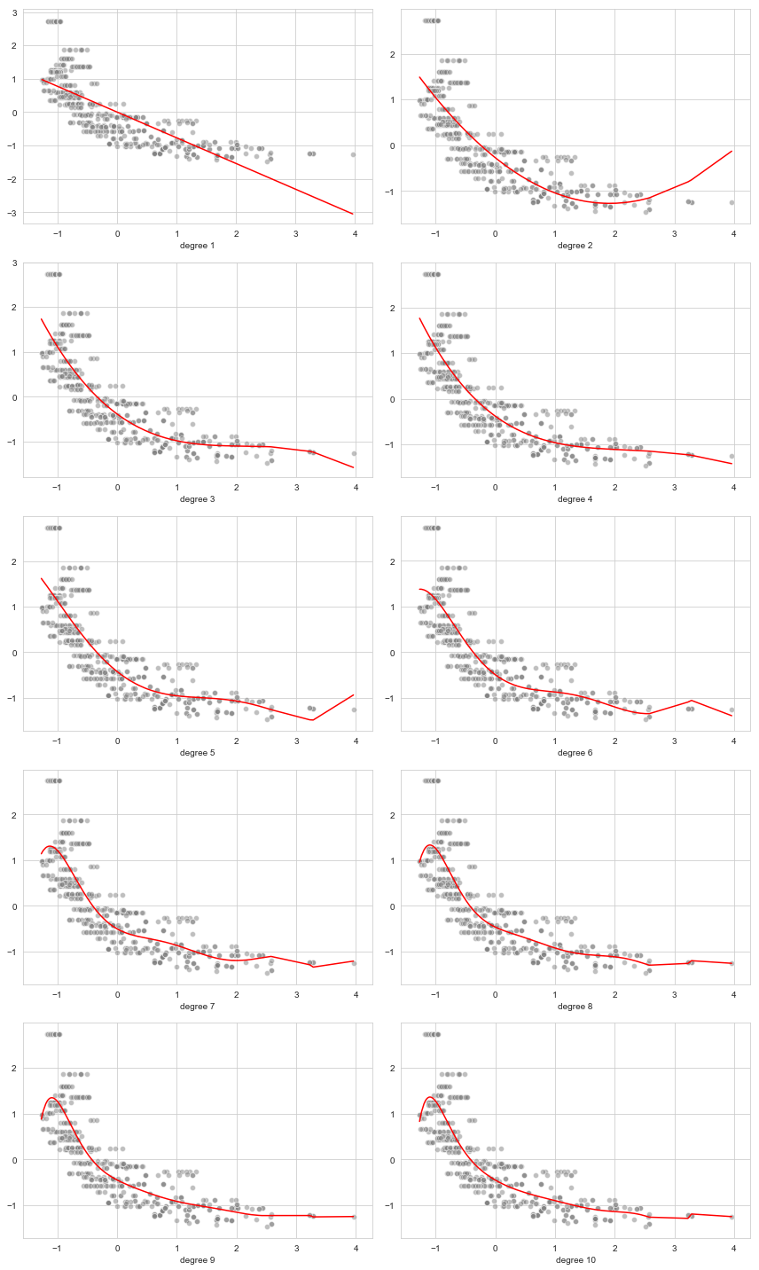
b. Polynomial regression for degree
regs = {d:None for d in range(1, 11)}

fig, axs = plt.subplots(nrows=5, ncols=2, figsize=(12,20))

for (i, d) in enumerate(regs):
    poly = PolynomialFeatures(degree=d)
    linreg = LinearRegression().fit(poly.fit_transform(X.reshape(-1, 1)), y)
    plt.subplot(5, 2, i + 1)
    sns.lineplot(x=X, y=linreg.predict(poly.fit_transform(X.reshape(-1,1))), color='red')
    sns.scatterplot(x=X, y=y, color='grey', alpha=0.5)
    plt.xlabel('degree ' + strd.)
    fig.tight_layout()
c. Optimizing the degree of the polynomial regression model
We’ll estimate the root mean squared error using 10-fold cross validation
from sklearn.pipeline import Pipeline
from sklearn.model_selection import GridSearchCV

poly_reg_pipe = Pipeline([('poly', PolynomialFeatures()), ('linreg', LinearRegression())])
poly_reg_params = {'poly__degree': np.arange(1, 10)}
poly_reg_search = GridSearchCV(estimator=poly_reg_pipe, param_grid=poly_reg_params, cv=10,
                               scoring='neg_mean_squared_error')
poly_reg_search.fit(X.reshape(-1, 1), y)
/anaconda3/lib/python3.7/site-packages/sklearn/model_selection/_search.py:841: DeprecationWarning: The default of the `iid` parameter will change from True to False in version 0.22 and will be removed in 0.24. This will change numeric results when test-set sizes are unequal.
  DeprecationWarning)


GridSearchCV(cv=10, error_score='raise-deprecating',
       estimator=Pipeline(memory=None,
     steps=[('poly', PolynomialFeatures(degree=2, include_bias=True, interaction_only=False)), ('linreg', LinearRegression(copy_X=True, fit_intercept=True, n_jobs=None,
         normalize=False))]),
       fit_params=None, iid='warn', n_jobs=None,
       param_grid={'poly__degree': array([1, 2, 3, 4, 5, 6, 7, 8, 9])},
       pre_dispatch='2*n_jobs', refit=True, return_train_score='warn',
       scoring='neg_mean_squared_error', verbose=0)
poly_reg_search.best_params_
{'poly__degree': 3}
np.sqrt(-poly_reg_search.best_score_)
0.5609950540561572
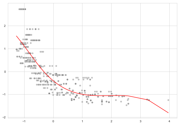
d. Cubic spline regression with 4 degrees of freedom
For this we’ll use patsy Python module. This blog post was helpful.
We’re using patsy.bs default choice for the knots (equally spaced quantiles), and default degree (3).
from patsy import dmatrix

X_tr = dmatrix("bs(x, df=4)", {'x': X})
spline_reg = LinearRegression()
spline_reg.fit(X_tr, y)
LinearRegression(copy_X=True, fit_intercept=True, n_jobs=None,
         normalize=False)
fig = plt.figure(figsize=(10, 7))
sns.lineplot(x=X, y=spline_reg.predict(X_tr), color='red')
sns.scatterplot(x=X, y=y, color='grey', alpha=0.5)
<matplotlib.axes._subplots.AxesSubplot at 0x1a2338a240>
from sklearn.metrics import mean_squared_error

np.sqrt(mean_squared_error(spline_reg.predict(X_tr), y))
0.5324989652537614
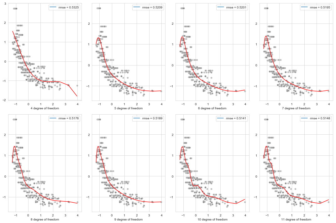
e. Cubic spline regression with degrees of freedom
fig, ax = plt.subplots(nrows=2, ncols=4, figsize=(15, 10))

for (i, d) in enumerate(range(4, 12)):

    X_tr = dmatrix("bs(x, df=" + strd. + ")", {'x': X})
    spline_reg = LinearRegression()
    spline_reg.fit(X_tr, y)
    rmse = round(np.sqrt(mean_squared_error(spline_reg.predict(X_tr), y)), 4)

    plt.subplot(2, 4, i + 1)
    sns.lineplot(x=X, y=spline_reg.predict(X_tr), color='red')
    plt.plot([], [], label='rmse = ' + str(rmse))
    sns.scatterplot(x=X, y=y, color='grey', alpha=0.5)
    plt.xlabel(strd. + ' degree of freedom')
    fig.tight_layout()
f. Optimizing the degrees of freedom of the cubic spline model
from sklearn.model_selection import cross_val_score

spline_cv_rmses = {d:None for d in range(4, 12)}

for d in spline_cv_rmses:
    X_tr = dmatrix("bs(x, df=" + strd. + ")", {'x': X})
    linreg = LinearRegression()
    cv_rmse = np.sqrt(-np.mean(cross_val_score(linreg,
                                               X_tr, y, cv=10,
                                               scoring='neg_mean_squared_error')))
    spline_cv_rmses[d] = cv_rmse

spline_cvs = pd.DataFrame({'dofs': list(spline_cv_rmses.keys()),
                           'cv_rmses': list(spline_cv_rmses.values())})
spline_cvs
| dofs | cv_rmses | |
|---|---|---|
| 0 | 4 | 0.632125 |
| 1 | 5 | 0.589646 |
| 2 | 6 | 0.592387 |
| 3 | 7 | 0.608314 |
| 4 | 8 | 0.629096 |
| 5 | 9 | 0.621942 |
| 6 | 10 | 0.640462 |
| 7 | 11 | 0.661658 |
fig = plt.figure(figsize=(10, 7))
sns.lineplot(x=spline_cvs['dofs'], y = spline_cvs['cv_rmses'], color='red')
<matplotlib.axes._subplots.AxesSubplot at 0x1a23c056a0>
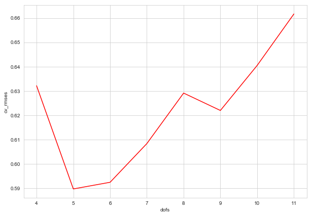
By cross-validation, (for this choice of knots), 5 is the best number of degrees of freedom