islr notes and exercises from An Introduction to Statistical Learning
7. Moving Beyond Linearity
Exercise 8: Investigating non-linear relationships in Auto dataset
Preparing the data
Import
# standard imports
%matplotlib inline
import matplotlib.pyplot as plt
import numpy as np
import pandas as pd
import seaborn as sns; sns.set()

auto = pd.read_csv('../../datasets/Auto.csv', index_col=0)
auto.head()
| mpg | cylinders | displacement | horsepower | weight | acceleration | year | origin | name | |
|---|---|---|---|---|---|---|---|---|---|
| 1 | 18.0 | 8 | 307.0 | 130 | 3504 | 12.0 | 70 | 1 | chevrolet chevelle malibu |
| 2 | 15.0 | 8 | 350.0 | 165 | 3693 | 11.5 | 70 | 1 | buick skylark 320 |
| 3 | 18.0 | 8 | 318.0 | 150 | 3436 | 11.0 | 70 | 1 | plymouth satellite |
| 4 | 16.0 | 8 | 304.0 | 150 | 3433 | 12.0 | 70 | 1 | amc rebel sst |
| 5 | 17.0 | 8 | 302.0 | 140 | 3449 | 10.5 | 70 | 1 | ford torino |
auto.info()
<class 'pandas.core.frame.DataFrame'>
Int64Index: 392 entries, 1 to 397
Data columns (total 9 columns):
mpg             392 non-null float64
cylinders       392 non-null int64
displacement    392 non-null float64
horsepower      392 non-null int64
weight          392 non-null int64
acceleration    392 non-null float64
year            392 non-null int64
origin          392 non-null int64
name            392 non-null object
dtypes: float64(3), int64(5), object(1)
memory usage: 30.6+ KB
Encode categorical variables
The only categorical (non-ordinal) variable is origin
# numerical df with one hot encoding for origin variable
auto_num = pd.get_dummies(auto, columns=['origin'])
auto_num.head()
| mpg | cylinders | displacement | horsepower | weight | acceleration | year | name | origin_1 | origin_2 | origin_3 | |
|---|---|---|---|---|---|---|---|---|---|---|---|
| 1 | 18.0 | 8 | 307.0 | 130 | 3504 | 12.0 | 70 | chevrolet chevelle malibu | 1 | 0 | 0 |
| 2 | 15.0 | 8 | 350.0 | 165 | 3693 | 11.5 | 70 | buick skylark 320 | 1 | 0 | 0 |
| 3 | 18.0 | 8 | 318.0 | 150 | 3436 | 11.0 | 70 | plymouth satellite | 1 | 0 | 0 |
| 4 | 16.0 | 8 | 304.0 | 150 | 3433 | 12.0 | 70 | amc rebel sst | 1 | 0 | 0 |
| 5 | 17.0 | 8 | 302.0 | 140 | 3449 | 10.5 | 70 | ford torino | 1 | 0 | 0 |
Inspecting the Data
Before training models we’ll do some inspection to see if non-linear relationships are suggested by the data.
A pairplot produces all possible scatterplots of the variables
# pair plot to inspect distributions and scatterplots
sns.pairplot(data=auto, diag_kind='kde', plot_kws={'alpha':0.5},
             diag_kws={'alpha':0.5})
<seaborn.axisgrid.PairGrid at 0x1a20dc77b8>
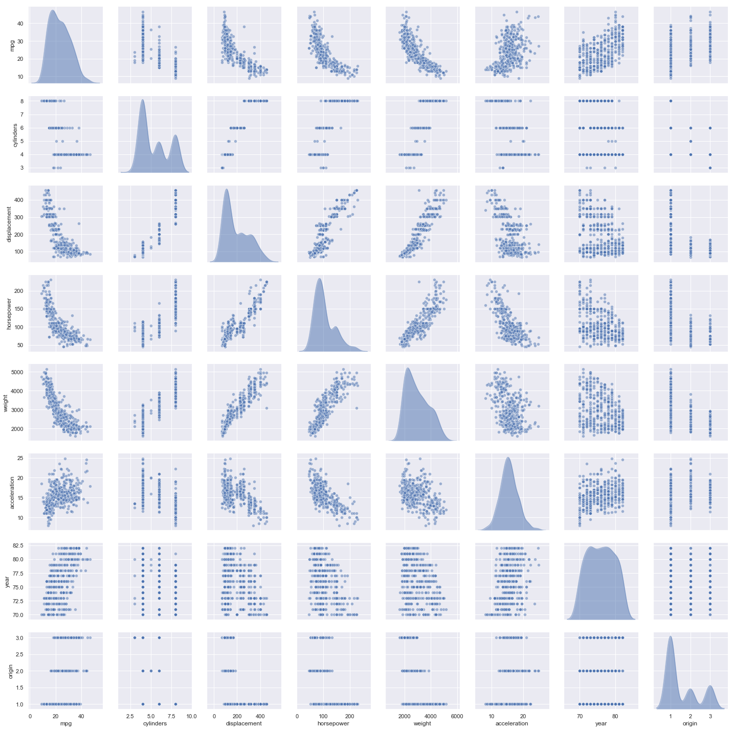
Observations:
- The plots strongly suggest that variables
weight,horsepoweranddisplacementhave non-linear relationships tompg - The plots weakly suggest that
displacementandhorsepowermay have a non-linear relationships toacceleration - There is strong suggestion of some linear relationships as well.
- It’s difficult to identify a non-linear relationship between two variables when one of them is discrete (e.g.
cylinders,year)
Modeling some non-linear relationships with mpg
Based on the pairplot we’ll investigate non-linear relationships between acceleration, weight, horsepower, and displacement with mpg. We’ll try a few different types of models, using cross-validation to optimize, and then compare
cols = ['acceleration', 'weight', 'horsepower', 'displacement', 'mpg']
df = auto[cols]

# normalize
df = (df - df.mean())/df.std()

# series
acc, wt, hp, dp, mpg = df.acceleration.values, df.weight.values, df.horsepower.values, df.displacement.values, df.mpg.values
Local Regression
from sklearn.neighbors import KNeighborsRegressor
from sklearn.model_selection import GridSearchCV

lr_param_grid = {'n_neighbors': np.arange(1,7), 'weights': ['uniform', 'distance'],
                     'p': np.arange(1, 7)}
lr_searches = [GridSearchCV(KNeighborsRegressor(), lr_param_grid, cv=5,
                         scoring='neg_mean_squared_error') for i in range(4)]
%%capture
var_pairs = {'acc_mpg', 'wt_mpg', 'hp_mpg', 'dp_mpg'}
models = {name:None for name in ['local', 'poly', 'p-spline']}

models['local'] = {pair:None for pair in var_pairs}
models['local']['acc_mpg'] = lr_searches[0].fit(acc.reshape(-1, 1), mpg)
models['local']['wt_mpg'] = lr_searches[1].fit(wt.reshape(-1, 1), mpg)
models['local']['hp_mpg'] = lr_searches[2].fit(hp.reshape(-1, 1), mpg)
models['local']['dp_mpg'] = lr_searches[3].fit(dp.reshape(-1, 1), mpg)
Polynomial Regression
from sklearn.pipeline import Pipeline
from sklearn.preprocessing import PolynomialFeatures
from sklearn.linear_model import Ridge
reg_tree_search.best_params_

# 6-fold cv estimate of test rmse
np.sqrt(-reg_tree_search.best_score_)

from sklearn.metrics import mean_squared_error

# test set mse
final_reg_tree = reg_tree_search.best_estimator_
reg_tree_test_mse = mean_squared_error(final_reg_tree.predict(X_test), y_test)
np.sqrt(reg_tree_test_mse)
pr_pipe = Pipeline(steps=[('poly', PolynomialFeatures()), ('ridge', Ridge())])
pr_pipe_param_grid = {'poly__degree': np.arange(1, 5), 'ridge__alpha': np.logspace(-4, 4, 5)}
pr_searches = [GridSearchCV(estimator=pr_pipe, param_grid=pr_pipe_param_grid, cv=5,
                              scoring='neg_mean_squared_error') for i in range(4)]
%%capture
models['poly'] = {pair:None for pair in var_pairs}
models['poly']['acc_mpg'] = pr_searches[0].fit(acc.reshape(-1, 1), mpg)
models['poly']['wt_mpg'] = pr_searches[1].fit(wt.reshape(-1, 1), mpg)
models['poly']['hp_mpg'] = pr_searches[2].fit(hp.reshape(-1, 1), mpg)
models['poly']['dp_mpg'] = pr_searches[3].fit(dp.reshape(-1, 1), mpg)
Cubic P-Spline Regression
Thankfully pygam’s GAM plays nice with sklearn’s GridSearchCV.
from pygam import GAM, s

gam = GAM(s(0))

ps_param_grid = {'n_splines': np.arange(10, 16), 'spline_order': np.arange(2, 4),
                 'lam': np.exp(np.random.rand(100, 1) * 6 - 3).flatten()}
ps_searches = [GridSearchCV(estimator=GAM(), param_grid=ps_param_grid, cv=5, scoring='neg_mean_squared_error')
               for i in range(4)]
Note that pygam.GAM.gridsearch uses generalized cross-validation (GCV).
%%capture
models['p-spline'] = {pair:None for pair in var_pairs}
models['p-spline']['acc_mpg'] = ps_searches[0].fit(acc.reshape(-1, 1), mpg)
models['p-spline']['wt_mpg'] = ps_searches[1].fit(wt.reshape(-1, 1), mpg)
models['p-spline']['hp_mpg'] = ps_searches[2].fit(hp.reshape(-1, 1), mpg)
models['p-spline']['dp_mpg'] = ps_searches[3].fit(dp.reshape(-1, 1), mpg)
Model Comparison
Optimal models and their test errors
cols = pd.MultiIndex.from_product([['acc_mpg', 'wt_mpg', 'hp_mpg', 'dp_mpg'], ['params', 'cv_mse']],
                                  names=['var_pair', 'opt_results'])
rows = pd.Index(['local', 'poly', 'p-spline'], name='model_type')

models_df = pd.DataFrame(index=rows, columns=cols)
models_df
| var_pair | acc_mpg | wt_mpg | hp_mpg | dp_mpg | ||||
|---|---|---|---|---|---|---|---|---|
| opt_results | params | cv_mse | params | cv_mse | params | cv_mse | params | cv_mse |
| model_type | ||||||||
| local | NaN | NaN | NaN | NaN | NaN | NaN | NaN | NaN |
| poly | NaN | NaN | NaN | NaN | NaN | NaN | NaN | NaN |
| p-spline | NaN | NaN | NaN | NaN | NaN | NaN | NaN | NaN |
for var_pair in models_df.columns.levels[0]:
    for name in models_df.index:
        models_df.loc[name, var_pair] = models[name][var_pair].best_params_, -models[name][var_pair].best_score_

models_df
| var_pair | acc_mpg | wt_mpg | hp_mpg | dp_mpg | ||||
|---|---|---|---|---|---|---|---|---|
| opt_results | params | cv_mse | params | cv_mse | params | cv_mse | params | cv_mse |
| model_type | ||||||||
| local | {'n_neighbors': 6, 'p': 1, 'weights': 'uniform'} | 1.02543 | {'n_neighbors': 6, 'p': 1, 'weights': 'uniform'} | 0.421562 | {'n_neighbors': 4, 'p': 1, 'weights': 'distance'} | 0.371018 | {'n_neighbors': 6, 'p': 1, 'weights': 'uniform'} | 0.406882 |
| poly | {'poly__degree': 4, 'ridge__alpha': 0.0001} | 0.969238 | {'poly__degree': 2, 'ridge__alpha': 0.0001} | 0.384849 | {'poly__degree': 2, 'ridge__alpha': 0.0001} | 0.399221 | {'poly__degree': 2, 'ridge__alpha': 0.0001} | 0.403257 |
| p-spline | {'lam': 3.1804238375997853, 'n_splines': 10, '... | 0.970488 | {'lam': 3.1804238375997853, 'n_splines': 10, '... | 0.391603 | {'lam': 3.1804238375997853, 'n_splines': 10, '... | 0.376321 | {'lam': 3.1804238375997853, 'n_splines': 10, '... | 0.392898 |
Analysis of optimal models
# helper for plotting results

def plot_results(var_name, var):
    fig, axes = plt.subplots(nrows=3, figsize=(10,10))

    for i, model_type in enumerate(models):
        model = models[model_type][var_name + '_mpg']
        plt.subplot(3, 1, i + 1)
        sns.lineplot(x=var, y=model.predict(var.reshape(-1, 1)), color='red',
                     label=model_type + " regression prediction")
        sns.scatterplot(x=var, y=mpg)
        plt.xlabel('std ' + var_name)
        plt.ylabel('std mpg')
        plt.legend()
        plt.tight_layout()
mpg vs accleration
The models seem to have much harder time predicting mpg from acceleration.
# mse estimates for acceleration models
models_df['acc_mpg']
| opt_results | params | cv_mse |
|---|---|---|
| model_type | ||
| local | {'n_neighbors': 6, 'p': 1, 'weights': 'uniform'} | 1.02543 |
| poly | {'poly__degree': 4, 'ridge__alpha': 0.0001} | 0.969238 |
| p-spline | {'lam': 3.1804238375997853, 'n_splines': 10, '... | 0.970488 |
plot_results('acc', acc)
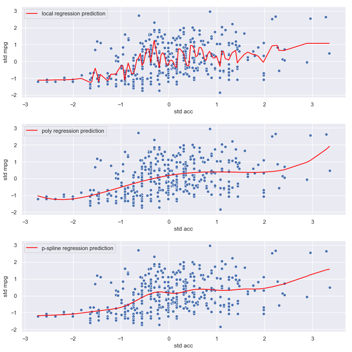
Observations:
- The local regression model seems to be fitting noise
- The polynomial and p-spline models are smoother, and less likely to overfit, which is consistent with their lower mse estimates
- The relationship between
accelerationandmpgappears weak
Conclusion:
There is little evidence of a relationship (linear or otherwise) between acceleration and mpg so we’ll omit acceleration from the final model
mpg vs. weight
# # mse estimates for acceleration models
models_df['wt_mpg']
| opt_results | params | cv_mse |
|---|---|---|
| model_type | ||
| local | {'n_neighbors': 6, 'p': 1, 'weights': 'uniform'} | 0.421562 |
| poly | {'poly__degree': 2, 'ridge__alpha': 0.0001} | 0.384849 |
| p-spline | {'lam': 3.1804238375997853, 'n_splines': 10, '... | 0.391603 |
plot_results('wt', wt)
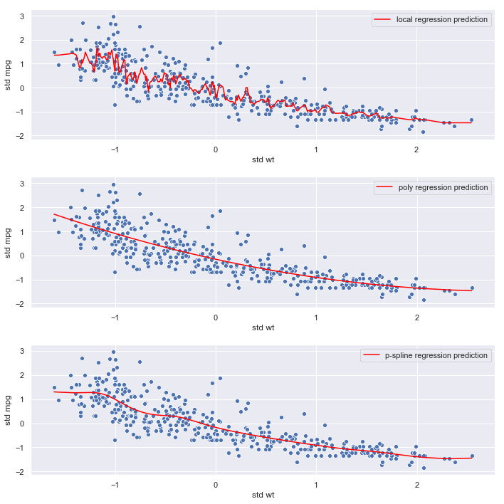
Observations:
- The local regression model again seems to be fitting noise
- The polynomial and p-spline models are smoother, and less likely to overfit, which is consistent with their lower mse estimates
- The relationship between
weightandmpgappears strong. - The p-spline and polynomial regression mses are very similar
models_df[('wt_mpg', 'params')]['poly']
{'poly__degree': 2, 'ridge__alpha': 0.0001}
models_df[('wt_mpg', 'params')]['p-spline']
{'lam': 3.1804238375997853, 'n_splines': 10, 'spline_order': 2}
Conclusion:
Optimal polynomial and p-spline models are both degree 2. Given its flexibility at the lower end of the range of weight, we’ll select the p-spline for the final model.
mpg vs. horsepower
# # mse estimates for acceleration models
models_df['hp_mpg']
| opt_results | params | cv_mse |
|---|---|---|
| model_type | ||
| local | {'n_neighbors': 4, 'p': 1, 'weights': 'distance'} | 0.371018 |
| poly | {'poly__degree': 2, 'ridge__alpha': 0.0001} | 0.399221 |
| p-spline | {'lam': 3.1804238375997853, 'n_splines': 10, '... | 0.376321 |
plot_results('hp', hp)
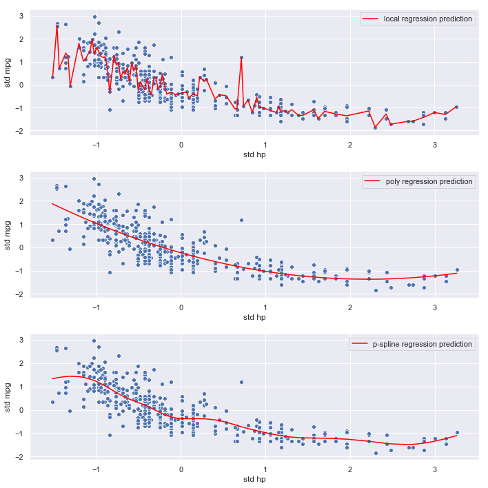
Observations:
- The local regression model again seems to be fitting noise
- The polynomial and p-spline models are smoother, and less likely to overfit, which is consistent with their lower mse estimates
- The relationship between
horsepowerandmpgappears strong. - The p-spline and polynomial regression mses are very similar
models_df[('hp_mpg', 'params')]['poly']
{'poly__degree': 2, 'ridge__alpha': 0.0001}
models_df[('hp_mpg', 'params')]['p-spline']
{'lam': 3.1804238375997853, 'n_splines': 10, 'spline_order': 2}
Conclusion:
Optimal polynomial and p-spline models are both degree 2. Given its flexibility at the lower end of the range of weight, we’ll select the p-spline for the final model.
mpg vs. displacement
# # mse estimates for acceleration models
models_df['dp_mpg']
| opt_results | params | cv_mse |
|---|---|---|
| model_type | ||
| local | {'n_neighbors': 6, 'p': 1, 'weights': 'uniform'} | 0.406882 |
| poly | {'poly__degree': 2, 'ridge__alpha': 0.0001} | 0.403257 |
| p-spline | {'lam': 3.1804238375997853, 'n_splines': 10, '... | 0.392898 |
plot_results('dp', dp)
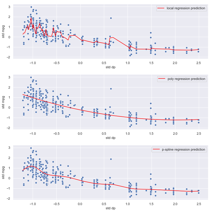
Observations:
- The local regression model again seems to be fitting noise
- The polynomial and p-spline models are smoother, and less likely to overfit, which is consistent with their lower mse estimates
- The relationship between
displacementandmpgappears strong. - The p-spline and polynomial regression mses are very similar
models_df[('dp_mpg', 'params')]['poly']
{'poly__degree': 2, 'ridge__alpha': 0.0001}
models_df[('dp_mpg', 'params')]['p-spline']
{'lam': 3.1804238375997853, 'n_splines': 10, 'spline_order': 2}
Conclusion:
Optimal polynomial and p-spline models are both degree 2. Given its flexibility at the lower end of the range of weight, we’ll select the p-spline for the final model.
GAM for predicting mpg
We identified some variables with non-linear relationships to mpg above, now we search for linear relationships. We’ll then fit a GAM which is a kind of hybrid model - linear on the linear variables, non-linear on the non-linear variables.
where the nonlinear functions are those found above.
Find variables with linear relationships to mpg
auto.corr()[auto.corr() > 0.5]
| mpg | cylinders | displacement | horsepower | weight | acceleration | year | origin | |
|---|---|---|---|---|---|---|---|---|
| mpg | 1.000000 | NaN | NaN | NaN | NaN | NaN | 0.580541 | 0.565209 |
| cylinders | NaN | 1.000000 | 0.950823 | 0.842983 | 0.897527 | NaN | NaN | NaN |
| displacement | NaN | 0.950823 | 1.000000 | 0.897257 | 0.932994 | NaN | NaN | NaN |
| horsepower | NaN | 0.842983 | 0.897257 | 1.000000 | 0.864538 | NaN | NaN | NaN |
| weight | NaN | 0.897527 | 0.932994 | 0.864538 | 1.000000 | NaN | NaN | NaN |
| acceleration | NaN | NaN | NaN | NaN | NaN | 1.0 | NaN | NaN |
| year | 0.580541 | NaN | NaN | NaN | NaN | NaN | 1.000000 | NaN |
| origin | 0.565209 | NaN | NaN | NaN | NaN | NaN | NaN | 1.000000 |
Train GAM
gam_df = auto_num.copy()

gam_df = gam_df.drop(columns=['acceleration', 'name'])
num_cols = ['mpg', 'cylinders', 'displacement', 'horsepower', 'weight', 'year']
gam_df.loc[: , num_cols] = (gam_df[num_cols] - gam_df[num_cols].mean()) / gam_df[num_cols].std()

gam_df.head()
| mpg | cylinders | displacement | horsepower | weight | year | origin_1 | origin_2 | origin_3 | |
|---|---|---|---|---|---|---|---|---|---|
| 1 | -0.697747 | 1.482053 | 1.075915 | 0.663285 | 0.619748 | -1.623241 | 1 | 0 | 0 |
| 2 | -1.082115 | 1.482053 | 1.486832 | 1.572585 | 0.842258 | -1.623241 | 1 | 0 | 0 |
| 3 | -0.697747 | 1.482053 | 1.181033 | 1.182885 | 0.539692 | -1.623241 | 1 | 0 | 0 |
| 4 | -0.953992 | 1.482053 | 1.047246 | 1.182885 | 0.536160 | -1.623241 | 1 | 0 | 0 |
| 5 | -0.825870 | 1.482053 | 1.028134 | 0.923085 | 0.554997 | -1.623241 | 1 | 0 | 0 |
from pygam import f

final_gam = GAM(s(1) + s(2) + s(3) + s(4) + s(5) + f(6) + f(7) + f(8))

ps_param_grid = {'n_splines': np.arange(15, 20), 'spline_order': np.arange(2, 3),
                 'lam': np.exp(np.random.rand(100, 1) * 6 - 3).flatten()}
ps_search = GridSearchCV(estimator=GAM(), param_grid=ps_param_grid, cv=10, scoring='neg_mean_squared_error')
ps_search.fit(gam_df.drop(columns=['mpg']), gam_df['mpg'])
/Users/home/anaconda3/lib/python3.6/site-packages/sklearn/model_selection/_search.py:841: DeprecationWarning: The default of the `iid` parameter will change from True to False in version 0.22 and will be removed in 0.24. This will change numeric results when test-set sizes are unequal.
  DeprecationWarning)


GridSearchCV(cv=10, error_score='raise-deprecating',
       estimator=GAM(callbacks=['deviance', 'diffs'], distribution='normal',
   fit_intercept=True, link='identity', max_iter=100, terms='auto',
   tol=0.0001, verbose=False),
       fit_params=None, iid='warn', n_jobs=None,
       param_grid={'n_splines': array([15, 16, 17, 18, 19]), 'spline_order': array([2]), 'lam': array([1.22679, 1.71212, ..., 0.19191, 0.68306])},
       pre_dispatch='2*n_jobs', refit=True, return_train_score='warn',
       scoring='neg_mean_squared_error', verbose=0)
Compare to alternative regression models
We’ll compare our GAM to to alternative null, ordinary least squares and polynomial ridge regression models.
from sklearn.dummy import DummyRegressor
from sklearn.linear_model import LinearRegression, Ridge
from sklearn.model_selection import cross_val_score

X, y = gam_df.drop(columns=['mpg']), gam_df['mpg']

# dummy model that always predicts mean response
dummy = DummyRegressor().fit(X, y)
dummy_cv_mse = np.mean(-cross_val_score(dummy, X, y, scoring='neg_mean_squared_error', cv=10))

# ordinary least squares
ols = LinearRegression().fit(X, y)
ols_cv_mse = np.mean(-cross_val_score(ols, X, y, scoring='neg_mean_squared_error', cv=10))

# optimized polynomial ridge
pr_pipe = Pipeline(steps=[('poly', PolynomialFeatures()), ('ridge', Ridge())])
pr_pipe_param_grid = {'poly__degree': np.arange(1, 5), 'ridge__alpha': np.logspace(-4, 4, 5)}
pr_search = GridSearchCV(estimator=pr_pipe, param_grid=pr_pipe_param_grid, cv=10,
                              scoring='neg_mean_squared_error')
ridge = pr_search.fit(X, y)
ridge_cv_mse = -ridge.best_score_

gam_cv_mse = -ps_search.best_score_
/Users/home/anaconda3/lib/python3.6/site-packages/sklearn/model_selection/_search.py:841: DeprecationWarning: The default of the `iid` parameter will change from True to False in version 0.22 and will be removed in 0.24. This will change numeric results when test-set sizes are unequal.
  DeprecationWarning)
comparison_df = pd.DataFrame({'cv_mse': [dummy_cv_mse, ols_cv_mse, ridge_cv_mse, gam_cv_mse]},
                             index=['dummy', 'ols', 'poly ridge', 'gam'])
comparison_df
| cv_mse | |
|---|---|
| dummy | 1.092509 |
| ols | 0.203995 |
| poly ridge | 0.127831 |
| gam | 0.201342 |
The polynomial ridge model has outperformed
ridge.best_params_
{'poly__degree': 3, 'ridge__alpha': 1.0}