7. Moving Beyond Linearity

Exercise 7: Using non-linear multiple regression to predict `wage` in `Wage` dataset

Preparing the data
Fitting some nonlinear models
Model Selection
Improvements

We’re modifying the exercise a bit to consider multiple regression (as opposed to considering different predictors individually). It’s not hard to see how the techniques of this chapter generalize to the multiple regression setting.

Preparing the data

Loading

%matplotlib inline
import numpy as np
import pandas as pd
import seaborn as sns; sns.set()

wage = pd.read_csv("../../datasets/Wage.csv")
wage.head()

	Unnamed: 0	year	age	maritl	race	education	region	jobclass	health	health_ins	logwage	wage
0	231655	2006	18	1. Never Married	1. White	1. < HS Grad	2. Middle Atlantic	1. Industrial	1. <=Good	2. No	4.318063	75.043154
1	86582	2004	24	1. Never Married	1. White	4. College Grad	2. Middle Atlantic	2. Information	2. >=Very Good	2. No	4.255273	70.476020
2	161300	2003	45	2. Married	1. White	3. Some College	2. Middle Atlantic	1. Industrial	1. <=Good	1. Yes	4.875061	130.982177
3	155159	2003	43	2. Married	3. Asian	4. College Grad	2. Middle Atlantic	2. Information	2. >=Very Good	1. Yes	5.041393	154.685293
4	11443	2005	50	4. Divorced	1. White	2. HS Grad	2. Middle Atlantic	2. Information	1. <=Good	1. Yes	4.318063	75.043154

wage.info()

<class 'pandas.core.frame.DataFrame'>
RangeIndex: 3000 entries, 0 to 2999
Data columns (total 12 columns):
Unnamed: 0    3000 non-null int64
year          3000 non-null int64
age           3000 non-null int64
maritl        3000 non-null object
race          3000 non-null object
education     3000 non-null object
region        3000 non-null object
jobclass      3000 non-null object
health        3000 non-null object
health_ins    3000 non-null object
logwage       3000 non-null float64
wage          3000 non-null float64
dtypes: float64(2), int64(3), object(7)
memory usage: 281.3+ KB

Cleaning

Drop columns

The unnamed column appears to be some sort of id number, which is useless for our purposes. We can also drop logwage since it’s redundant

wage = wage.drop(columns=['Unnamed: 0', 'logwage'])

Convert to numerical dtypes

wage_num = pd.get_dummies(wage)
wage_num.head()

	year	age	wage	maritl_1. Never Married	maritl_2. Married	maritl_4. Divorced	race_1. White	...	education_3. Some College	education_4. College Grad	region_2. Middle Atlantic	jobclass_1. Industrial	jobclass_2. Information	health_1. <=Good	health_2. >=Very Good	health_ins_1. Yes	health_ins_2. No
0	2006	18	75.043154	1	0	0	1	...	0	0	1	1	0	1	0	0	1
1	2004	24	70.476020	1	0	0	1	...	0	1	1	0	1	0	1	0	1
2	2003	45	130.982177	0	1	0	1	...	1	0	1	1	0	1	0	1	0
3	2003	43	154.685293	0	1	0	0	...	0	1	1	0	1	0	1	1	0
4	2005	50	75.043154	0	0	1	1	...	0	0	1	0	1	1	0	1	0

5 rows × 24 columns

Preprocessing

Scaling the numerical variables

df = wage_num[['year', 'age', 'wage']]
wage_num_std = wage_num.copy()
wage_num_std.loc[:, ['year', 'age', 'wage']] = (df - df.mean())/df.std()
wage_num_std.head()

	year	age	wage	maritl_1. Never Married	maritl_2. Married	maritl_4. Divorced	race_1. White	...	education_3. Some College	education_4. College Grad	region_2. Middle Atlantic	jobclass_1. Industrial	jobclass_2. Information	health_1. <=Good	health_2. >=Very Good	health_ins_1. Yes	health_ins_2. No
0	0.103150	-2.115215	-0.878545	1	0	0	1	...	0	0	1	1	0	1	0	0	1
1	-0.883935	-1.595392	-0.987994	1	0	0	1	...	0	1	1	0	1	0	1	0	1
2	-1.377478	0.223986	0.461999	0	1	0	1	...	1	0	1	1	0	1	0	1	0
3	-1.377478	0.050712	1.030030	0	1	0	0	...	0	1	1	0	1	0	1	1	0
4	-0.390392	0.657171	-0.878545	0	0	1	1	...	0	0	1	0	1	1	0	1	0

5 rows × 24 columns

Fitting some nonlinear models

X_sc, y_sc = wage_num_std.drop(columns=['wage']).values, wage_num_std['wage'].values

X_sc.shape, y_sc.shape

((3000, 23), (3000,))

Polynomial Ridge Regression

We don’t need a special module for this model - we can use a scikit-learn pipeline.

We’ll use 10-fold cross validation to pick the polynomial degree and L2 penalty.

from sklearn.preprocessing import PolynomialFeatures
from sklearn.pipeline import Pipeline
from sklearn.linear_model import Ridge

pr_pipe = Pipeline([('poly', PolynomialFeatures()), ('ridge', Ridge())])
pr_param_grid = dict(poly__degree=np.arange(1, 5), ridge__alpha=np.logspace(-4, 4, 5))
pr_search = GridSearchCV(pr_pipe, pr_param_grid, cv=5, scoring='neg_mean_squared_error')
pr_search.fit(X_sc, y_sc)

GridSearchCV(cv=5, error_score='raise-deprecating',
       estimator=Pipeline(memory=None,
     steps=[('poly', PolynomialFeatures(degree=2, include_bias=True, interaction_only=False)), ('ridge', Ridge(alpha=1.0, copy_X=True, fit_intercept=True, max_iter=None,
   normalize=False, random_state=None, solver='auto', tol=0.001))]),
       fit_params=None, iid='warn', n_jobs=None,
       param_grid={'poly__degree': array([1, 2, 3, 4]), 'ridge__alpha': array([1.e-04, 1.e-02, 1.e+00, 1.e+02, 1.e+04])},
       pre_dispatch='2*n_jobs', refit=True, return_train_score='warn',
       scoring='neg_mean_squared_error', verbose=0)

pr_search.best_params_

{'poly__degree': 2, 'ridge__alpha': 100.0}

Local Regression

scikit-learn has support for local regression

from sklearn.neighbors import KNeighborsRegressor
from sklearn.model_selection import GridSearchCV

lr_param_grid = dict(n_neighbors=np.arange(1,7), weights=['uniform', 'distance'], 
                     p=np.arange(1, 7))
lr_search = GridSearchCV(KNeighborsRegressor(), lr_param_grid, cv=10, 
                         scoring='neg_mean_squared_error')
lr_search.fit(X_sc, y_sc)

GridSearchCV(cv=10, error_score='raise-deprecating',
       estimator=KNeighborsRegressor(algorithm='auto', leaf_size=30, metric='minkowski',
          metric_params=None, n_jobs=None, n_neighbors=5, p=2,
          weights='uniform'),
       fit_params=None, iid='warn', n_jobs=None,
       param_grid={'n_neighbors': array([1, 2, 3, 4, 5, 6]), 'weights': ['uniform', 'distance'], 'p': array([1, 2, 3, 4, 5, 6])},
       pre_dispatch='2*n_jobs', refit=True, return_train_score='warn',
       scoring='neg_mean_squared_error', verbose=0)

lr_search.best_params_

{'n_neighbors': 6, 'p': 1, 'weights': 'uniform'}

GAMs

GAMs are quite general. There exists python modules that implement specific choices for the nonlinear component functions $f_i(X_i)$ . Here we’ll explore two modules that seem relatively mature/well-maintained.

GAMs with `pyGAM`

The module pyGAM implements P-splines.

from pygam import GAM, s, f

# generate string for terms
spline_terms = ' + '.join(['s(' + stri. + ')' for i in range(0,3)])
factor_terms = ' + '.join(['f(' + stri. + ')' 
                           for i in range(3,X_sc.shape[1])])
terms = spline_terms + ' + ' + factor_terms
terms

's(0) + s(1) + s(2) + f(3) + f(4) + f(5) + f(6) + f(7) + f(8) + f(9) + f(10) + f(11) + f(12) + f(13) + f(14) + f(15) + f(16) + f(17) + f(18) + f(19) + f(20) + f(21) + f(22)'

pygam_gam = GAM(s(0) + s(1) + s(2) + f(3) + f(4) + f(5) + f(6) + f(7) 
                + f(8) + f(9) + f(10) + f(11) + f(12) + f(13) + f(14) 
                + f(15) + f(16) + f(17) + f(18) + f(19) + f(20) + f(21) 
                + f(22))

ps_search = pygam_gam.gridsearch(X_sc, y_sc, progress=True, 
                     lam=np.exp(np.random.rand(100, 23) * 6 - 3))

100% (100 of 100) |######################| Elapsed Time: 0:00:13 Time:  0:00:13

Model Selection

As in exercise 6, we’ll select a model on the basis of mean squared test error.

mse_test_df = pd.DataFrame({'mse_test':np.zeros(3)}, index=['poly_ridge', 'local_reg', 'p_spline'])

# polynomial ridge and local regression models already have CV estimates of test mse
mse_test_df.at['poly_ridge', 'mse_test'] = -pr_search.best_score_
mse_test_df.at['local_reg', 'mse_test'] = -lr_search.best_score_

from sklearn.model_selection import cross_val_score

# get p-spline CV estimate of test mse
mse_test_df.at['p_spline', 'mse_test'] = -np.mean(cross_val_score(ps_search,
                                                                  X_sc, y_sc, scoring='neg_mean_squared_error',
                                                                  cv=10))

mse_test_df

	mse_test
poly_ridge	0.653614
local_reg	0.741645
p_spline	1.000513

Polynomial ridge regression has won out. Since this CV mse estimate was calculated on scaled data, let’s get the estimate for the original data

%%capture
X, y = wage_num.drop(columns=['wage']).values, wage_num['wage'].values
cv_score = cross_val_score(pr_search.best_estimator_, X, y, scoring='neg_mean_squared_error', cv=10)

mse = -np.mean(cv_score)
mse

1137.2123862552992

me = np.sqrt(mse)
me

33.722579768684646

sns.distplot(wage['wage'])

<matplotlib.axes._subplots.AxesSubplot at 0x1a20d1e668>

png

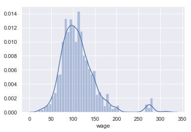
wage['wage'].describe()

count    3000.000000
mean      111.703608
std        41.728595
min        20.085537
25%        85.383940
50%       104.921507
75%       128.680488
max       318.342430
Name: wage, dtype: float64

This model predicts a mean (absolute) error of $~\approx 33.7$

print('{}'.format(round(me/wage['wage'].std(), 2)))

0.81

which is 0.81 standard deviations.

Improvements

After inspecting the distribution of wage, it’s fairly clear there is a group of outliers that are no doubt affecting the prediction accuracy of the model. Let’s try to separate that group.

sns.scatterplot(x=wage.index, y=wage['wage'].sort_values(), alpha=0.4, color='grey')

<matplotlib.axes._subplots.AxesSubplot at 0x1a2469d8d0>

png

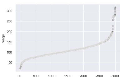
There appears to be a break point around 250. Let’s take all rows with wage less than this

wage_num_low = wage_num[wage_num['wage'] < 250]
wage_num_low_sc = wage_num_low.copy()

df = wage_num_low_sc[['year', 'age', 'wage']]
wage_num_low_sc.loc[:, ['year', 'age', 'wage']] = (df - df.mean())/df.std()

Let train the same models again

X_low_sc, y_low_sc = wage_num_low_sc.drop(columns=['wage']).values, wage_num_low_sc['wage']

# polynomial ridge model
pr_search.fit(X_low_sc, y_low_sc)

/Users/home/anaconda3/lib/python3.6/site-packages/sklearn/model_selection/_search.py:841: DeprecationWarning: The default of the `iid` parameter will change from True to False in version 0.22 and will be removed in 0.24. This will change numeric results when test-set sizes are unequal.
  DeprecationWarning)





GridSearchCV(cv=5, error_score='raise-deprecating',
       estimator=Pipeline(memory=None,
     steps=[('poly', PolynomialFeatures(degree=2, include_bias=True, interaction_only=False)), ('ridge', Ridge(alpha=1.0, copy_X=True, fit_intercept=True, max_iter=None,
   normalize=False, random_state=None, solver='auto', tol=0.001))]),
       fit_params=None, iid='warn', n_jobs=None,
       param_grid={'poly__degree': array([1, 2, 3, 4]), 'ridge__alpha': array([1.e-04, 1.e-02, 1.e+00, 1.e+02, 1.e+04])},
       pre_dispatch='2*n_jobs', refit=True, return_train_score='warn',
       scoring='neg_mean_squared_error', verbose=0)

pr_search.best_params_

{'poly__degree': 2, 'ridge__alpha': 100.0}

# local regression
lr_search.fit(X_low_sc, y_low_sc)

GridSearchCV(cv=10, error_score='raise-deprecating',
       estimator=KNeighborsRegressor(algorithm='auto', leaf_size=30, metric='minkowski',
          metric_params=None, n_jobs=None, n_neighbors=5, p=2,
          weights='uniform'),
       fit_params=None, iid='warn', n_jobs=None,
       param_grid={'n_neighbors': array([1, 2, 3, 4, 5, 6]), 'weights': ['uniform', 'distance'], 'p': array([1, 2, 3, 4, 5, 6])},
       pre_dispatch='2*n_jobs', refit=True, return_train_score='warn',
       scoring='neg_mean_squared_error', verbose=0)

lr_search.best_params_

{'n_neighbors': 6, 'p': 5, 'weights': 'uniform'}

# p spline 
ps_search = pygam_gam.gridsearch(X_low_sc, y_low_sc, progress=True, 
                     lam=np.exp(np.random.rand(100, 23) * 6 - 3))

100% (100 of 100) |######################| Elapsed Time: 0:00:25 Time:  0:00:25

ps_search.summary()

GAM                                                                                                       
=============================================== ==========================================================
Distribution:                        NormalDist Effective DoF:                                     28.9895
Link Function:                     IdentityLink Log Likelihood:                                 -3606.1899
Number of Samples:                         2921 AIC:                                             7272.3587
                                                AICc:                                            7273.0018
                                                GCV:                                                0.6157
                                                Scale:                                              0.6047
                                                Pseudo R-Squared:                                   0.4011
==========================================================================================================
Feature Function                  Lambda               Rank         EDoF         P > x        Sig. Code   
================================= ==================== ============ ============ ============ ============
s(0)                              [13.8473]            20           7.0          1.38e-05     ***         
s(1)                              [17.046]             20           8.3          3.52e-13     ***         
s(2)                              [0.1439]             20           1.1          5.30e-04     ***         
f(3)                              [11.8899]            2            1.0          3.09e-02     *           
f(4)                              [3.5507]             2            0.9          2.96e-01                 
f(5)                              [0.1322]             2            0.9          1.79e-02     *           
f(6)                              [14.0907]            2            0.0          3.22e-01                 
f(7)                              [8.8878]             2            1.0          2.87e-01                 
f(8)                              [0.2954]             2            1.0          3.01e-01                 
f(9)                              [2.0563]             2            0.9          6.03e-01                 
f(10)                             [8.6475]             2            0.0          3.51e-01                 
f(11)                             [8.7695]             2            1.0          1.11e-16     ***         
f(12)                             [0.1363]             2            1.0          2.69e-02     *           
f(13)                             [0.9965]             2            1.0          1.11e-16     ***         
f(14)                             [0.1233]             2            1.0          1.11e-16     ***         
f(15)                             [0.3011]             2            0.0          1.11e-16     ***         
f(16)                             [2.094]              1            0.0          1.00e+00                 
f(17)                             [0.6317]             2            1.0          2.06e-01                 
f(18)                             [16.422]             2            0.0          2.07e-01                 
f(19)                             [0.3865]             2            1.0          1.33e-05     ***         
f(20)                             [4.8438]             2            0.0          1.38e-05     ***         
f(21)                             [0.1626]             2            1.0          1.11e-16     ***         
f(22)                             [0.3707]             2            0.0          1.11e-16     ***         
intercept                                              1            0.0          2.88e-01                 
==========================================================================================================
Significance codes:  0 '***' 0.001 '**' 0.01 '*' 0.05 '.' 0.1 ' ' 1

WARNING: Fitting splines and a linear function to a feature introduces a model identifiability problem
         which can cause p-values to appear significant when they are not.

WARNING: p-values calculated in this manner behave correctly for un-penalized models or models with
         known smoothing parameters, but when smoothing parameters have been estimated, the p-values
         are typically lower than they should be, meaning that the tests reject the null too readily.


/Users/home/anaconda3/lib/python3.6/site-packages/ipykernel_launcher.py:1: UserWarning: KNOWN BUG: p-values computed in this summary are likely much smaller than they should be. 
 
Please do not make inferences based on these values! 

Collaborate on a solution, and stay up to date at: 
github.com/dswah/pyGAM/issues/163 

  """Entry point for launching an IPython kernel.

low_mse_test_df = pd.DataFrame({'low_mse_test':np.zeros(3)}, index=['poly_ridge', 'local_reg', 'p_spline'])
low_mse_test_df.at['poly_ridge', 'low_mse_test'] = -pr_search.best_score_
low_mse_test_df.at['local_reg', 'low_mse_test'] = -lr_search.best_score_
low_mse_test_df.at['p_spline', 'low_mse_test'] = -np.mean(cross_val_score(ps_search,
                                                                 X_low_sc, y_low_sc, scoring='neg_mean_squared_error',
                                                                 cv=10))
mse_df = pd.concat([mse_test_df, low_mse_test_df], axis=1)
mse_df

	mse_test	low_mse_test
poly_ridge	0.653614	0.613098
local_reg	0.741645	0.701615
p_spline	1.000513	1.000513

There was a considerable improvement for the polynomial ridge and local regression models.

islr notes and exercises from An Introduction to Statistical Learning