islr notes and exercises from An Introduction to Statistical Learning
7. Moving Beyond Linearity
Exercise 6: Using polynomial and step function regression to predict wage using age in Wage dataset
Preparing the data
%matplotlib inline
import numpy as np
import pandas as pd
import seaborn as sns; sns.set()

wage = pd.read_csv("../../datasets/Wage.csv")
wage.head()
| Unnamed: 0 | year | age | maritl | race | education | region | jobclass | health | health_ins | logwage | wage | |
|---|---|---|---|---|---|---|---|---|---|---|---|---|
| 0 | 231655 | 2006 | 18 | 1. Never Married | 1. White | 1. < HS Grad | 2. Middle Atlantic | 1. Industrial | 1. <=Good | 2. No | 4.318063 | 75.043154 |
| 1 | 86582 | 2004 | 24 | 1. Never Married | 1. White | 4. College Grad | 2. Middle Atlantic | 2. Information | 2. >=Very Good | 2. No | 4.255273 | 70.476020 |
| 2 | 161300 | 2003 | 45 | 2. Married | 1. White | 3. Some College | 2. Middle Atlantic | 1. Industrial | 1. <=Good | 1. Yes | 4.875061 | 130.982177 |
| 3 | 155159 | 2003 | 43 | 2. Married | 3. Asian | 4. College Grad | 2. Middle Atlantic | 2. Information | 2. >=Very Good | 1. Yes | 5.041393 | 154.685293 |
| 4 | 11443 | 2005 | 50 | 4. Divorced | 1. White | 2. HS Grad | 2. Middle Atlantic | 2. Information | 1. <=Good | 1. Yes | 4.318063 | 75.043154 |
wage.info()
<class 'pandas.core.frame.DataFrame'>
RangeIndex: 3000 entries, 0 to 2999
Data columns (total 12 columns):
Unnamed: 0    3000 non-null int64
year          3000 non-null int64
age           3000 non-null int64
maritl        3000 non-null object
race          3000 non-null object
education     3000 non-null object
region        3000 non-null object
jobclass      3000 non-null object
health        3000 non-null object
health_ins    3000 non-null object
logwage       3000 non-null float64
wage          3000 non-null float64
dtypes: float64(2), int64(3), object(7)
memory usage: 281.3+ KB
a. Predict wage with age using polynomial regression with L2 penalty.
See sklearn docs on polynomial regression. We’re going to add an L2 penalty for fun (and performance improvement)
from sklearn.preprocessing import PolynomialFeatures, scale
from sklearn.linear_model import Ridge
from sklearn.pipeline import Pipeline
from sklearn.model_selection import GridSearchCV

steps = [('poly', PolynomialFeatures()), ('ridge', Ridge())]
pipe = Pipeline(steps=steps)
param_grid = dict(poly__degree=np.arange(1, 5), ridge__alpha=np.logspace(-4, 4, 5))
search = GridSearchCV(pipe, param_grid, cv=10, scoring='neg_mean_squared_error')
%%capture

X, y = wage['age'], wage['wage']
X_sc, y_sc = scale(wage['age']), scale(wage['wage'])
search.fit(X_sc.reshape(-1, 1), y_sc)
The best 10-fold CV model has parameters
search.best_params_
{'poly__degree': 4, 'ridge__alpha': 1.0}
This model has a CV mse test error estimate of
-search.best_score_
0.9156879981745668
This represents an absolute error of
np.sqrt(-search.best_score_)
0.9569158783166715
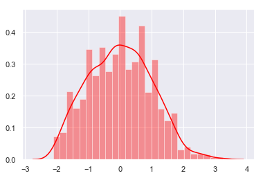
Not terribly good - this is about one standard deviation (since the data were normalized)
sns.distplot(X_sc, color='red')
<matplotlib.axes._subplots.AxesSubplot at 0x1a1effe6a0>
Now to use these parameters on the original data to get a real mse test reading
from sklearn.model_selection import train_test_split
from sklearn.metrics import mean_squared_error

X_poly = PolynomialFeatures(degree=4).fit_transform(X.values.reshape(-1,1))
X_train, X_test, y_train, y_test = train_test_split(X_poly, y, test_size=0.33, random_state=42)
ridge = Ridge(alpha=1).fit(X_train, y_train)
np.sqrt(mean_squared_error(y_test, ridge.predict(X_test)))
/Users/home/anaconda3/lib/python3.6/site-packages/sklearn/linear_model/ridge.py:125: LinAlgWarning: Ill-conditioned matrix (rcond=2.01369e-17): result may not be accurate.
  overwrite_a=True).T


39.239871740545624
We’ll plot the model fitted curve against the original data
t = np.linspace(X.min(), X.max(), 3000)
y_pred = ridge.predict(PolynomialFeatures(degree=4).fit_transform(t.reshape(-1,1)))

sns.lineplot(t, y_pred, color='red')
sns.scatterplot(X, y, color='grey', alpha=0.4)
<matplotlib.axes._subplots.AxesSubplot at 0x1a1ebe6e48>

b. Predict wage with age using step function regression
Sklearn doesn’t have a builtin for step functions, so we’ll use basis-expansions, a Python module by Matthew Drury (cf his blog post for an accessible discussion of basis expansions).
from basis_expansions import Binner
from sklearn.linear_model import LinearRegression

bin_reg = dict(n_cuts=[], mse_test=[])

X_sc_train, X_sc_test, y_sc_train, y_sc_test = train_test_split(X_sc, y_sc, test_size=0.33)

for n_cuts in range(1, 26):
    bin_reg['n_cuts'] += [n_cuts]

    steps = [('bin', Binner(X_sc.min(), X_sc.max(), n_cuts=n_cuts)), ('linreg', LinearRegression(fit_intercept=False))]
    pipe_fit = Pipeline(steps=steps).fit(X_sc_train, y_sc_train)
    bin_reg['mse_test'] += [mean_squared_error(y_sc_test, pipe_fit.predict(X_sc_test))]
bin_reg_df = pd.DataFrame(bin_reg)
sns.lineplot(x=bin_reg_df['n_cuts'], y=bin_reg_df['mse_test'], color='red')
<matplotlib.axes._subplots.AxesSubplot at 0x1a1eef7588>
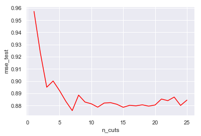
bin_reg_df.loc[bin_reg_df['mse_test'].idxmin(), :]
n_cuts      7.000000
mse_test    0.875825
Name: 6, dtype: float64
X_train, X_test, y_train, y_test = train_test_split(X.values.reshape(-1,1), y, test_size=0.33, random_state=42)
binner = Binner(X.min(), X.max(), n_cuts=7)
linreg = LinearRegression(fit_intercept=False).fit(binner.fit_transform(X_train), y_train)
np.sqrt(mean_squared_error(y_test, linreg.predict(binner.fit_transform(X_test))))
39.24772730694755
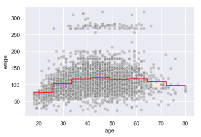
t = np.linspace(X.min(), X.max(), 3000)
y_pred = linreg.predict(binner.fit_transform(t.reshape(-1,1)))

sns.lineplot(t, y_pred, color='red')
sns.scatterplot(X, y, color='grey', alpha=0.4)
<matplotlib.axes._subplots.AxesSubplot at 0x1a1ef712e8>