islr notes and exercises from An Introduction to Statistical Learning
6. Linear Model Selection and Regularization
Exercise 9: Predicting Apps in College dataset
Preparing the data
import pandas as pd

college = pd.read_csv('../../datasets/College.csv')
college = college.rename({'Unnamed: 0': 'Name'}, axis='columns')
college.head()
| Name | Private | Apps | Accept | Enroll | Top10perc | Top25perc | F.Undergrad | P.Undergrad | Outstate | Room.Board | Books | Personal | PhD | Terminal | S.F.Ratio | perc.alumni | Expend | Grad.Rate | |
|---|---|---|---|---|---|---|---|---|---|---|---|---|---|---|---|---|---|---|---|
| 0 | Abilene Christian University | Yes | 1660 | 1232 | 721 | 23 | 52 | 2885 | 537 | 7440 | 3300 | 450 | 2200 | 70 | 78 | 18.1 | 12 | 7041 | 60 |
| 1 | Adelphi University | Yes | 2186 | 1924 | 512 | 16 | 29 | 2683 | 1227 | 12280 | 6450 | 750 | 1500 | 29 | 30 | 12.2 | 16 | 10527 | 56 |
| 2 | Adrian College | Yes | 1428 | 1097 | 336 | 22 | 50 | 1036 | 99 | 11250 | 3750 | 400 | 1165 | 53 | 66 | 12.9 | 30 | 8735 | 54 |
| 3 | Agnes Scott College | Yes | 417 | 349 | 137 | 60 | 89 | 510 | 63 | 12960 | 5450 | 450 | 875 | 92 | 97 | 7.7 | 37 | 19016 | 59 |
| 4 | Alaska Pacific University | Yes | 193 | 146 | 55 | 16 | 44 | 249 | 869 | 7560 | 4120 | 800 | 1500 | 76 | 72 | 11.9 | 2 | 10922 | 15 |
college.loc[:, 'Private'] = [0 if entry == 'No' else 1 for entry in college['Private']]
college.info()
<class 'pandas.core.frame.DataFrame'>
RangeIndex: 777 entries, 0 to 776
Data columns (total 19 columns):
Name           777 non-null object
Private        777 non-null int64
Apps           777 non-null int64
Accept         777 non-null int64
Enroll         777 non-null int64
Top10perc      777 non-null int64
Top25perc      777 non-null int64
F.Undergrad    777 non-null int64
P.Undergrad    777 non-null int64
Outstate       777 non-null int64
Room.Board     777 non-null int64
Books          777 non-null int64
Personal       777 non-null int64
PhD            777 non-null int64
Terminal       777 non-null int64
S.F.Ratio      777 non-null float64
perc.alumni    777 non-null int64
Expend         777 non-null int64
Grad.Rate      777 non-null int64
dtypes: float64(1), int64(17), object(1)
memory usage: 115.4+ KB
a. Train - test split
from sklearn.model_selection import train_test_split

X_train, X_test, y_train, y_test = train_test_split(college.drop(columns=['Apps', 'Name']),
                                                    college['Apps'])
b. Linear regression model
from sklearn.linear_model import LinearRegression
from sklearn.metrics import mean_squared_error

linreg = LinearRegression().fit(X_train, y_train)
linreg_mse_test = mean_squared_error(y_test, linreg.predict(X_test))
mses_df = pd.DataFrame({'mse_test': linreg_mse_test},
                       index=['linreg'])
mses_df
| mse_test | |
|---|---|
| linreg | 1.869641e+06 |
c. Ridge regression model
from sklearn.linear_model import Ridge
from sklearn.model_selection import GridSearchCV

parameters = {'alpha': [10**i for i in range(-3, 4)]}
ridge = GridSearchCV(Ridge(), parameters, cv=10,
                     scoring='neg_mean_squared_error')
%%capture

ridge.fit(X_train, y_train)
%%capture

ridge_cv_df = pd.DataFrame(ridge.cv_results_)
ridge_cv_df
ridge_mse_test = mean_squared_error(y_test, ridge.best_estimator_.predict(X_test))
mses_df = mses_df.append(pd.DataFrame({'mse_test': ridge_mse_test}, index=['ridge']))
mses_df
| mse_test | |
|---|---|
| linreg | 1.869641e+06 |
| ridge | 1.875181e+06 |
d. Lasso regression model
from sklearn.linear_model import Lasso
from sklearn.model_selection import GridSearchCV

parameters = {'alpha': [10**i for i in range(-3, 4)]}
lasso = GridSearchCV(Lasso(), parameters, cv=10, scoring='neg_mean_squared_error')
%%capture

lasso.fit(X_train, y_train)
%%capture

lasso_cv_df = pd.DataFrame(lasso.cv_results_)
lasso_cv_df
lasso_mse_test = mean_squared_error(y_test, lasso.best_estimator_.predict(X_test))
mses_df = mses_df.append(pd.DataFrame({'mse_test': lasso_mse_test}, index=['lasso']))
mses_df
| mse_test | |
|---|---|
| linreg | 1.869641e+06 |
| ridge | 1.875181e+06 |
| lasso | 1.870846e+06 |
e. PCR model
scikit-learn doesn’t have combined PCA and regression so we’ll use the top answer to this CrossValidated question
import numpy as np
from sklearn.preprocessing import scale
from sklearn.decomposition import PCA
from sklearn.model_selection import cross_val_score
n = len(X_train_reduced)
linreg = LinearRegression()

pcr_mses = [-cross_val_score(linreg, np.ones((n,1)), y_train, cv=10,
                         scoring='neg_mean_squared_error').mean()]
for i in range(1, college.shape[1] - b1):
    pcr_mses += [-cross_val_score(linreg, X_train_reduced[:, :i], y_train, cv=10,
                              scoring='neg_mean_squared_error').mean()]
np.argmin(pcr_mses)
17
10 fold Cross-validation selects (full PCR model with no intercept).
pcr = LinearRegression().fit(X_train.iloc[:, :np.argmin(pcr_mses)], y_train)
The test error of this model is
pcr_mse_test = mean_squared_error(y_test, pcr.predict(X_test))
mses_df = mses_df.append(pd.DataFrame({'mse_test': pcr_mse_test}, index=['pcr']))
mses_df
| mse_test | |
|---|---|
| linreg | 1.869641e+06 |
| ridge | 1.875181e+06 |
| lasso | 1.870846e+06 |
| pcr | 1.869641e+06 |
f. PLS model
from sklearn.cross_decomposition import PLSRegression

# mse for only constant predictor same as for pcr
pls_mses = pcr_mses[:1]

for i in range(1, college.shape[1] - 1):
    pls_mses += [-cross_val_score(estimator=PLSRegression(n_components = i),
                                  X=X_train, y=y_train, cv=10,
                                  scoring='neg_mean_squared_error').mean()]
np.argmin(pls_mses)
13
10 fold CV selects
pls = PLSRegression(n_components=13).fit(X_train, y_train)
pls_mse_test = mean_squared_error(y_test, pls.predict(X_test))
mses_df = mses_df.append(pd.DataFrame({'mse_test': pls_mse_test}, index=['pls']))
mses_df
| mse_test | |
|---|---|
| linreg | 1.869641e+06 |
| ridge | 1.875181e+06 |
| lasso | 1.870846e+06 |
| pcr | 1.869641e+06 |
| pls | 1.862860e+06 |
g. Comments
How accurately can we predict applications?
The test mses for each model were . This corresponds to an (absolute) error of . Given the distribution of applications
college['Apps'].describe()
count      777.000000
mean      3001.638353
std       3870.201484
min         81.000000
25%        776.000000
50%       1558.000000
75%       3624.000000
max      48094.000000
Name: Apps, dtype: float64
import seaborn as sns

% matplotlib inline

sns.distplot(college['Apps'])
<matplotlib.axes._subplots.AxesSubplot at 0x1a212479b0>
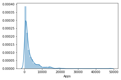
The prediction doesn’t seem that accurate. Given that distribution is highly concentrated about the mean and the upper quartile is , we can say that for most values, the prediction is off by of the true value.
Is there much difference among the test errors
No