islr notes and exercises from An Introduction to Statistical Learning
6. Linear Model Selection and Regularization
Exercise 8: Feature Selection on Simulated Data
a. Generate predictor and noise
import numpy as np

X, e = np.random.normal(size=100), np.random.normal(size=100)
X.shape
(100,)
b. Generate response
(beta_0, beta_1, beta_2, beta_3) = 1, 1, 1, 1

y = beta_0*np.array(100*[1]) + beta_1*X + beta_2*X**2 + beta_2*X**3 + e
import matplotlib.pyplot as plt
import seaborn as sns
%matplotlib inline
sns.set()
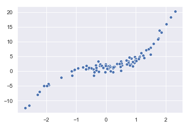
sns.scatterplot(x=X, y=y)
<matplotlib.axes._subplots.AxesSubplot at 0x1a186bed68>
c. Best Subset Selection
First we generate the predictors and assemble all data in a dataframe
import pandas as pd

data = pd.DataFrame({'X^' + stri.: X**i for i in range(11)})
data['y'] = y
data.head()
| X^0 | X^1 | X^2 | X^3 | X^4 | X^5 | X^6 | X^7 | X^8 | X^9 | X^10 | y | |
|---|---|---|---|---|---|---|---|---|---|---|---|---|
| 0 | 1.0 | 0.115404 | 0.013318 | 0.001537 | 0.000177 | 0.000020 | 0.000002 | 2.726196e-07 | 3.146150e-08 | 3.630796e-09 | 4.190099e-10 | 1.914734 |
| 1 | 1.0 | -0.594583 | 0.353530 | -0.210203 | 0.124983 | -0.074313 | 0.044185 | -2.627180e-02 | 1.562078e-02 | -9.287856e-03 | 5.522406e-03 | 0.848536 |
| 2 | 1.0 | 1.751695 | 3.068436 | 5.374965 | 9.415301 | 16.492737 | 28.890250 | 5.060691e+01 | 8.864789e+01 | 1.552841e+02 | 2.720104e+02 | 11.091760 |
| 3 | 1.0 | -0.662284 | 0.438620 | -0.290491 | 0.192387 | -0.127415 | 0.084385 | -5.588676e-02 | 3.701289e-02 | -2.451304e-02 | 1.623459e-02 | 1.893104 |
| 4 | 1.0 | -1.921016 | 3.690302 | -7.089130 | 13.618332 | -26.161034 | 50.255764 | -9.654213e+01 | 1.854590e+02 | -3.562696e+02 | 6.843997e+02 | -4.628707 |
The mlxtend library has exhaustive feature selection
from sklearn.linear_model import LinearRegression
from sklearn.metrics import mean_squared_error
from mlxtend.feature_selection import ExhaustiveFeatureSelector as EFS

# dict for results
bss = {}

for k in range(1, 12):
    reg = LinearRegression()
    efs = EFS(reg,
               min_features=k,
               max_features=k,
               scoring='neg_mean_squared_error',
               print_progress=False,
               cv=None)
    efs = efs.fit(data.drop(columns=['y']), data['y'])
    bss[k] = efs.best_idx_

bss
{1: (3,),
 2: (2, 3),
 3: (1, 2, 3),
 4: (1, 2, 3, 7),
 5: (1, 2, 3, 9, 10),
 6: (1, 2, 3, 6, 8, 9),
 7: (1, 2, 3, 6, 7, 9, 10),
 8: (1, 2, 3, 4, 6, 8, 9, 10),
 9: (1, 2, 4, 5, 6, 7, 8, 9, 10),
 10: (1, 2, 3, 4, 5, 6, 7, 8, 9, 10),
 11: (0, 1, 2, 3, 4, 5, 6, 7, 8, 9, 10)}
Now we’ll calculate and adjusted for each subset size and plot (We’ll use instead of since they’re proportional).
First some helper functions for and adjusted
from math import log

def AIC(n, rss, d, var_e):
    return (1 / (n * var_e)) * (rss + 2 * d * var_e)

def BIC(n, rss, d, var_e):
    return (1 / (n * var_e)) * (rss + log(n) * d * var_e)

def adj_r2(n, rss, tss, d):
    return 1 - ((rss / (n - d - 1)) / (tss / (n - 1)))
Then calculate
def mse_estimates(X, y, bss):
    n, results = X.shape[1], {}
    for k in bss:
        model_fit = LinearRegression().fit(X[:, bss[k]], y)
        y_pred = model_fit.predict(X[:, bss[k]])

        errors = y - y_pred
        rss = np.dot(errors, errors)
        var_e = np.var(errors)
        tss = np.dot((y - np.mean(y)), (y - np.mean(y)))

        results[k] = dict(AIC=AIC(n, rss, k, var_e), BIC=BIC(n, rss, k, var_e),
                          adj_r2=adj_r2(n, rss, rss, k))
    return results
X, y = data.drop(columns=['y']).values, data['y'].values
mses = mse_estimates(X, y, bss)
mses
/Users/home/anaconda3/lib/python3.6/site-packages/ipykernel_launcher.py:10: RuntimeWarning: divide by zero encountered in double_scalars
  # Remove the CWD from sys.path while we load stuff.


{1: {'AIC': 9.272727272727272,
  'BIC': 9.308899570254397,
  'adj_r2': -0.11111111111111094},
 2: {'AIC': 9.454545454545455, 'BIC': 9.526890049599706, 'adj_r2': -0.25},
 3: {'AIC': 9.636363636363633,
  'BIC': 9.744880528945009,
  'adj_r2': -0.4285714285714284},
 4: {'AIC': 9.81818181818182,
  'BIC': 9.962871008290318,
  'adj_r2': -0.6666666666666665},
 5: {'AIC': 10.0, 'BIC': 10.180861487635624, 'adj_r2': -1.0},
 6: {'AIC': 10.181818181818185, 'BIC': 10.398851966980931, 'adj_r2': -1.5},
 7: {'AIC': 10.363636363636365,
  'BIC': 10.616842446326237,
  'adj_r2': -2.3333333333333335},
 8: {'AIC': 10.545454545454545, 'BIC': 10.834832925671542, 'adj_r2': -4.0},
 9: {'AIC': 10.727272727272727, 'BIC': 11.05282340501685, 'adj_r2': -9.0},
 10: {'AIC': 10.909090909090908, 'BIC': 11.270813884362154, 'adj_r2': -inf},
 11: {'AIC': 11.090909090909093, 'BIC': 11.488804363707464, 'adj_r2': 11.0}}
AICs = np.array([mses[k]['AIC'] for k in mses])
BICs = np.array([mses[k]['BIC'] for k in mses])
adj_r2s = np.array([mses[k]['adj_r2'] for k in mses])
x = np.arange(1, 12)
sns.lineplot(x, AICs)
sns.lineplot(x, BICs)
sns.lineplot(x, adj_r2s)
<matplotlib.axes._subplots.AxesSubplot at 0x1a1980a668>
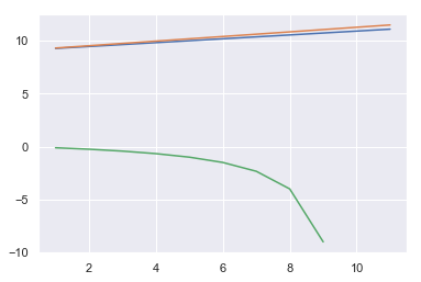
The best model has the highest AIC/BIC and lowest adjusted , so on this basis, the model with the only feature is the best.
The coefficient is:
bss_model = LinearRegression().fit(X[:, 3].reshape(-1, 1), y)
bss_model.coef_
array([1.06262895])
Now, lets generate a validataion data set and check this model’s mse
X_valid, e_valid = np.random.normal(size=100), np.random.normal(size=100)
(beta_0, beta_1, beta_2, beta_3) = 1, 1, 1, 1
y_valid = beta_0*np.array(100*[1]) + beta_1*X_valid + beta_2*X_valid**2 + beta_2*X_valid**3 + e
y_pred = bss_model.coef_ * X_valid**3
errors = y_pred - y_valid
bss_mse_test = np.mean(np.dot(errors, errors))
bss_mse_test
642.7014227682031
We’ll save the results for later comparison
model_selection_df = pd.DataFrame({'mse_test': [bss_mse_test]}, index=['bss'])
model_selection_df
| mse_test | |
|---|---|
| bss | 642.701423 |
d. Forward and Backward Stepwise Selection
mlxtend also has forward and backward stepwise selection
First we look at forward stepwise selection.
from mlxtend.feature_selection import SequentialFeatureSelector as SFS

X, y = data.drop(columns=['y']).values, data['y'].values
# dict for results
fss = {}

for k in range(1, 12):
    sfs = SFS(LinearRegression(),
          k_features=k,
          forward=True,
          floating=False,
          scoring='neg_mean_squared_error')
    sfs = sfs.fit(X, y)
    fss[k] = sfs.k_feature_idx_

fss
{1: (3,),
 2: (2, 3),
 3: (1, 2, 3),
 4: (1, 2, 3, 9),
 5: (0, 1, 2, 3, 9),
 6: (0, 1, 2, 3, 9, 10),
 7: (0, 1, 2, 3, 5, 9, 10),
 8: (0, 1, 2, 3, 4, 5, 9, 10),
 9: (0, 1, 2, 3, 4, 5, 7, 9, 10),
 10: (0, 1, 2, 3, 4, 5, 7, 8, 9, 10),
 11: (0, 1, 2, 3, 4, 5, 6, 7, 8, 9, 10)}
mses = mse_estimates(X, y, fss)
mses
/Users/home/anaconda3/lib/python3.6/site-packages/ipykernel_launcher.py:10: RuntimeWarning: divide by zero encountered in double_scalars
  # Remove the CWD from sys.path while we load stuff.


{1: {'AIC': 9.272727272727272,
  'BIC': 9.308899570254397,
  'adj_r2': -0.11111111111111094},
 2: {'AIC': 9.454545454545455, 'BIC': 9.526890049599706, 'adj_r2': -0.25},
 3: {'AIC': 9.636363636363633,
  'BIC': 9.744880528945009,
  'adj_r2': -0.4285714285714284},
 4: {'AIC': 9.818181818181818,
  'BIC': 9.962871008290316,
  'adj_r2': -0.6666666666666667},
 5: {'AIC': 10.0, 'BIC': 10.180861487635623, 'adj_r2': -1.0},
 6: {'AIC': 10.181818181818182, 'BIC': 10.39885196698093, 'adj_r2': -1.5},
 7: {'AIC': 10.363636363636365,
  'BIC': 10.616842446326237,
  'adj_r2': -2.3333333333333335},
 8: {'AIC': 10.545454545454547, 'BIC': 10.834832925671542, 'adj_r2': -4.0},
 9: {'AIC': 10.727272727272727, 'BIC': 11.052823405016847, 'adj_r2': -9.0},
 10: {'AIC': 10.90909090909091, 'BIC': 11.270813884362157, 'adj_r2': -inf},
 11: {'AIC': 11.090909090909093, 'BIC': 11.488804363707464, 'adj_r2': 11.0}}
AICs = np.array([mses[k]['AIC'] for k in mses])
BICs = np.array([mses[k]['BIC'] for k in mses])
adj_r2s = np.array([mses[k]['adj_r2'] for k in mses])
x = np.arange(1, 12)
sns.lineplot(x, AICs)
sns.lineplot(x, BICs)
sns.lineplot(x, adj_r2s)
<matplotlib.axes._subplots.AxesSubplot at 0x1a198f0d68>

FSS also selects the model with the only feature.
Now we consider backward stepwise selection.
from mlxtend.feature_selection import SequentialFeatureSelector as SFS

# dict for results
bkss = {}

for k in range(1, 12):
    sfs = SFS(LinearRegression(),
          k_features=k,
          forward=False,
          floating=False,
          scoring='neg_mean_squared_error')
    sfs = sfs.fit(X, y)
    bkss[k] = sfs.k_feature_idx_

bkss
{1: (3,),
 2: (2, 3),
 3: (1, 2, 3),
 4: (1, 2, 3, 9),
 5: (1, 2, 3, 8, 9),
 6: (1, 2, 3, 7, 8, 9),
 7: (1, 2, 3, 6, 7, 8, 9),
 8: (0, 1, 2, 3, 6, 7, 8, 9),
 9: (0, 1, 2, 3, 5, 6, 7, 8, 9),
 10: (0, 1, 2, 3, 5, 6, 7, 8, 9, 10),
 11: (0, 1, 2, 3, 4, 5, 6, 7, 8, 9, 10)}
mses = mse_estimates(X, y, bkss)
mses
/Users/home/anaconda3/lib/python3.6/site-packages/ipykernel_launcher.py:10: RuntimeWarning: divide by zero encountered in double_scalars
  # Remove the CWD from sys.path while we load stuff.


{1: {'AIC': 9.272727272727272,
  'BIC': 9.308899570254397,
  'adj_r2': -0.11111111111111094},
 2: {'AIC': 9.454545454545455, 'BIC': 9.526890049599706, 'adj_r2': -0.25},
 3: {'AIC': 9.636363636363633,
  'BIC': 9.744880528945009,
  'adj_r2': -0.4285714285714284},
 4: {'AIC': 9.818181818181818,
  'BIC': 9.962871008290316,
  'adj_r2': -0.6666666666666667},
 5: {'AIC': 10.0, 'BIC': 10.180861487635623, 'adj_r2': -1.0},
 6: {'AIC': 10.181818181818182, 'BIC': 10.398851966980928, 'adj_r2': -1.5},
 7: {'AIC': 10.363636363636363,
  'BIC': 10.616842446326235,
  'adj_r2': -2.333333333333333},
 8: {'AIC': 10.545454545454543, 'BIC': 10.83483292567154, 'adj_r2': -4.0},
 9: {'AIC': 10.727272727272725, 'BIC': 11.052823405016847, 'adj_r2': -9.0},
 10: {'AIC': 10.90909090909091, 'BIC': 11.270813884362155, 'adj_r2': -inf},
 11: {'AIC': 11.090909090909093, 'BIC': 11.488804363707464, 'adj_r2': 11.0}}
AICs = np.array([mses[k]['AIC'] for k in mses])
BICs = np.array([mses[k]['BIC'] for k in mses])
adj_r2s = np.array([mses[k]['adj_r2'] for k in mses])
x = np.arange(1, 12)
sns.lineplot(x, AICs)
sns.lineplot(x, BICs)
sns.lineplot(x, adj_r2s)
<matplotlib.axes._subplots.AxesSubplot at 0x1a199cccc0>

BKSS also selects the model with the only feature.
e. Lasso
from sklearn.linear_model import Lasso
from sklearn.model_selection import cross_val_score
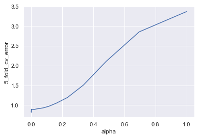
alphas = np.array([10**i for i in np.linspace(-3, 0, num=20)])
lassos = {'alpha': alphas, '5_fold_cv_error': []}
for alpha in alphas:
        lasso = Lasso(alpha=alpha, fit_intercept=False, max_iter=1e8, tol=1e-2)
        cv_error = np.mean(- cross_val_score(lasso, X, y, cv=5,
                                             scoring='neg_mean_squared_error'))
        lassos['5_fold_cv_error'] += [cv_error]
lassos_df = pd.DataFrame(lassos)
lassos_df
| alpha | 5_fold_cv_error | |
|---|---|---|
| 0 | 0.001000 | 0.836428 |
| 1 | 0.001438 | 0.819378 |
| 2 | 0.002069 | 0.895901 |
| 3 | 0.002976 | 0.893177 |
| 4 | 0.004281 | 0.888498 |
| 5 | 0.006158 | 0.885597 |
| 6 | 0.008859 | 0.884861 |
| 7 | 0.012743 | 0.884489 |
| 8 | 0.018330 | 0.888298 |
| 9 | 0.026367 | 0.894860 |
| 10 | 0.037927 | 0.906162 |
| 11 | 0.054556 | 0.914259 |
| 12 | 0.078476 | 0.930345 |
| 13 | 0.112884 | 0.968640 |
| 14 | 0.162378 | 1.049202 |
| 15 | 0.233572 | 1.192103 |
| 16 | 0.335982 | 1.506187 |
| 17 | 0.483293 | 2.109461 |
| 18 | 0.695193 | 2.854881 |
| 19 | 1.000000 | 3.368783 |
(alpha_hat, cv_error_min) = lassos_df.iloc[lassos_df['5_fold_cv_error'].idxmin(), ]
(alpha_hat, cv_error_min)
(0.0014384498882876629, 0.8193781004864231)
sns.lineplot(x='alpha', y='5_fold_cv_error', data=lassos_df)
<matplotlib.axes._subplots.AxesSubplot at 0x1a19a8b5c0>
Now we’ll see what coefficient estimates this model produces
np.set_printoptions(suppress=True)
lasso_model = Lasso(alpha=alpha_hat, fit_intercept=False, max_iter=1e8, tol=1e-2).fit(X, y)
lasso_model.coef_
array([ 1.06544938,  0.80612409,  2.05979396,  0.7883535 , -1.66945357,
        0.24562823,  0.76952192, -0.0535788 , -0.13390294,  0.0027605 ,
        0.00767839])
model_df = pd.DataFrame({'coef_': lasso_model.coef_}, index=data.columns[:-1])
model_df.sort_values(by='coef_', ascending=False)
| coef_ | |
|---|---|
| X^2 | 2.059794 |
| X^0 | 1.065449 |
| X^1 | 0.806124 |
| X^3 | 0.788354 |
| X^6 | 0.769522 |
| X^5 | 0.245628 |
| X^10 | 0.007678 |
| X^9 | 0.002760 |
| X^7 | -0.053579 |
| X^8 | -0.133903 |
| X^4 | -1.669454 |
Let’s check this model on a validation set:
data_valid = pd.DataFrame({'X_valid^' + stri.: X_valid**i for i in range(11)})
data_valid['y_valid'] = y_valid
data_valid.head()
| X_valid^0 | X_valid^1 | X_valid^2 | X_valid^3 | X_valid^4 | X_valid^5 | X_valid^6 | X_valid^7 | X_valid^8 | X_valid^9 | X_valid^10 | y_valid | |
|---|---|---|---|---|---|---|---|---|---|---|---|---|
| 0 | 1.0 | 1.315735 | 1.731159 | 2.277747 | 2.996911 | 3.943142 | 5.188130 | 6.826205 | 8.981478 | 11.817247 | 15.548367 | 7.109116 |
| 1 | 1.0 | 0.754402 | 0.569123 | 0.429348 | 0.323901 | 0.244352 | 0.184340 | 0.139066 | 0.104912 | 0.079146 | 0.059708 | 3.052666 |
| 2 | 1.0 | 0.910262 | 0.828578 | 0.754223 | 0.686541 | 0.624932 | 0.568852 | 0.517805 | 0.471338 | 0.429041 | 0.390540 | 3.389726 |
| 3 | 1.0 | -0.528947 | 0.279785 | -0.147991 | 0.078279 | -0.041406 | 0.021901 | -0.011585 | 0.006128 | -0.003241 | 0.001714 | 2.010106 |
| 4 | 1.0 | -1.271336 | 1.616296 | -2.054856 | 2.612413 | -3.321256 | 4.222433 | -5.368133 | 6.824703 | -8.676493 | 11.030740 | -1.018760 |
y_pred = lasso_model.predict(data_valid.drop(columns=['y_valid']))
errors = y_pred - y_valid
lasso_mse_test = np.mean(np.dot(errors, errors))
lasso_mse_test
90.33155498089704
model_selection_df = model_selection_df.append(pd.DataFrame({'mse_test': [lasso_mse_test]}, index=['lasso']))
model_selection_df
| mse_test | |
|---|---|
| bss | 642.701423 |
| lasso | 90.331555 |
A considerable improvement over the BSS model
f. Repeat for a new response
We now repeat the above for a model
New response
# new train/test response
y = np.array(100*[1]) + data['X^7'] + e

# new validation response
y_valid = np.array(100*[1]) + data_valid['X_valid^7'] + e

# update dfs
data.loc[:, 'y'], data_valid.loc[:, 'y_valid'] = y, y_valid
BSS model
bss = {}

for k in range(1, 12):
    reg = LinearRegression()
    efs = EFS(reg,
               min_features=k,
               max_features=k,
               scoring='neg_mean_squared_error',
               print_progress=False,
               cv=None)
    efs = efs.fit(data.drop(columns=['y']), data['y'])
    bss[k] = efs.best_idx_

bss
{1: (7,),
 2: (7, 9),
 3: (1, 3, 7),
 4: (1, 5, 7, 10),
 5: (1, 7, 8, 9, 10),
 6: (1, 4, 6, 7, 8, 9),
 7: (2, 4, 6, 7, 8, 9, 10),
 8: (1, 2, 4, 5, 6, 7, 8, 10),
 9: (2, 3, 4, 5, 6, 7, 8, 9, 10),
 10: (1, 2, 3, 4, 5, 6, 7, 8, 9, 10),
 11: (0, 1, 2, 3, 4, 5, 6, 7, 8, 9, 10)}
X, y = data.drop(columns=['y']).values, data['y'].values
mses = mse_estimates(X, y, bss)
mses
/Users/home/anaconda3/lib/python3.6/site-packages/ipykernel_launcher.py:10: RuntimeWarning: divide by zero encountered in double_scalars
  # Remove the CWD from sys.path while we load stuff.


{1: {'AIC': 9.272727272727272,
  'BIC': 9.308899570254397,
  'adj_r2': -0.11111111111111116},
 2: {'AIC': 9.454545454545455, 'BIC': 9.526890049599706, 'adj_r2': -0.25},
 3: {'AIC': 9.636363636363637,
  'BIC': 9.74488052894501,
  'adj_r2': -0.4285714285714286},
 4: {'AIC': 9.818181818181817,
  'BIC': 9.962871008290316,
  'adj_r2': -0.6666666666666667},
 5: {'AIC': 10.000000000000002, 'BIC': 10.180861487635623, 'adj_r2': -1.0},
 6: {'AIC': 10.18181818181818, 'BIC': 10.398851966980928, 'adj_r2': -1.5},
 7: {'AIC': 10.363636363636365,
  'BIC': 10.616842446326238,
  'adj_r2': -2.3333333333333335},
 8: {'AIC': 10.545454545454547, 'BIC': 10.834832925671542, 'adj_r2': -4.0},
 9: {'AIC': 10.727272727272723, 'BIC': 11.052823405016845, 'adj_r2': -9.0},
 10: {'AIC': 10.909090909090908, 'BIC': 11.270813884362154, 'adj_r2': -inf},
 11: {'AIC': 11.090909090909088, 'BIC': 11.488804363707459, 'adj_r2': 11.0}}
AICs = np.array([mses[k]['AIC'] for k in mses])
BICs = np.array([mses[k]['BIC'] for k in mses])
adj_r2s = np.array([mses[k]['adj_r2'] for k in mses])
x = np.arange(1, 12)
sns.lineplot(x, AICs)
sns.lineplot(x, BICs)
sns.lineplot(x, adj_r2s)
<matplotlib.axes._subplots.AxesSubplot at 0x1a1a241c18>

Again, BSS likes a single predictor (this time )
bss_model = LinearRegression().fit(data['X^7'].values.reshape(-1,1), data['y'].values)
bss_model.coef_
array([0.99897181])
Now, lets generate a validataion data set and check this model’s mse
y_pred = bss_model.coef_ * X_valid**3
errors = y_pred - y_valid
bss_mse_test = np.mean(np.dot(errors, errors))
bss_mse_test
91636.16819263707
model_selection_df = pd.DataFrame({'mse_test': [bss_mse_test]}, index=['bss'])
model_selection_df
| mse_test | |
|---|---|
| bss | 91636.168193 |
Lasso model
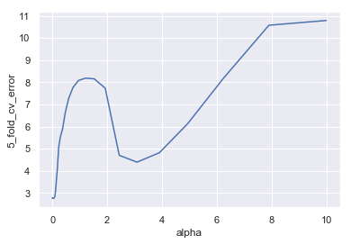
alphas = np.array([10**i for i in np.linspace(-4, 1, num=50)])
lassos = {'alpha': alphas, '5_fold_cv_error': []}

for alpha in alphas:
        lasso = Lasso(alpha=alpha, fit_intercept=False, max_iter=1e6, tol=1e-3)
        cv_error = np.mean(- cross_val_score(lasso, X, y, cv=5,
                                             scoring='neg_mean_squared_error'))
        lassos['5_fold_cv_error'] += [cv_error]
(alpha, cv_error_min) = lassos_df.iloc[lassos_df['5_fold_cv_error'].idxmin(), ]
(alpha, cv_error_min)
(0.028117686979742307, 2.750654968384496)
lassos_df = pd.DataFrame(lassos)
sns.lineplot(x='alpha', y='5_fold_cv_error', data=lassos_df)
<matplotlib.axes._subplots.AxesSubplot at 0x1a1a120da0>
Now we’ll see what coefficient estimates this model produces
lasso_model = Lasso(alpha=alpha, fit_intercept=False, max_iter=1e8, tol=1e-2).fit(X, y)
lasso_model.coef_
array([-0.        ,  1.43769581,  4.23293404, -4.72479707, -1.3268075 ,
        2.69250184, -0.02715976,  0.40441206,  0.01230247,  0.04725243,
        0.00255472])
model_df = pd.DataFrame({'coef_': lasso_model.coef_}, index=data.columns[:-1])
model_df.sort_values(by='coef_', ascending=False)
| coef_ | |
|---|---|
| X^2 | 4.232934 |
| X^5 | 2.692502 |
| X^1 | 1.437696 |
| X^7 | 0.404412 |
| X^9 | 0.047252 |
| X^8 | 0.012302 |
| X^10 | 0.002555 |
| X^0 | -0.000000 |
| X^6 | -0.027160 |
| X^4 | -1.326808 |
| X^3 | -4.724797 |
y_pred = lasso_model.predict(data_valid.drop(columns=['y_valid']))
errors = y_pred - y_valid
lasso_mse_test = np.mean(np.dot(errors, errors))
lasso_mse_test
292.261615448788
model_selection_df = model_selection_df.append(pd.DataFrame({'mse_test': [lasso_mse_test]}, index=['lasso']))
model_selection_df
| mse_test | |
|---|---|
| bss | 91636.168193 |
| lasso | 292.261615 |
Once again, the lasso dramatically outperforms.