5. Resampling Methods

Exercise 8: Cross-validation on simulated data

a. Generate data
b. Scatter plot
c. LOOCV errors for various models
d. Repeat c.
- e. Which model had the smallest error?
- f. Hypothesis testing the coefficients

a. Generate data

import numpy as np

np.random.seed(0)

X = np.random.normal(size=100)
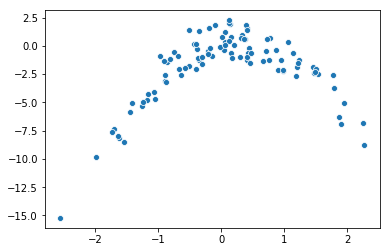
Y = -2*X**2 + X + np.random.normal(size=100)

The model here is

$Y = -2 X^2 + X + \epsilon$

Where $X, \epsilon \sim \text{Normal}(0, 1)$ .

The sample size is $n=100$ . Since we don’t know polynomial regression yet, we have $p=2$ , i.e. $X_1 = X, X_2 = X^2$ .

b. Scatter plot

import seaborn as sns
%matplotlib inline

sns.scatterplot(X, Y)

<matplotlib.axes._subplots.AxesSubplot at 0x1a1f70d4e0>

png

c. LOOCV errors for various models

Dataframe

import pandas as pd

data = pd.DataFrame({'const': len(X)*[1], 'X': X, 'Y': Y})
for i in range(2,5):
    data['X_' + stri.] = X**i

data.head()

	const	X	Y	X_2	X_3	X_4
0	1	1.764052	-2.576558	3.111881	5.489520	9.683801
1	1	0.400157	-1.267853	0.160126	0.064075	0.025640
2	1	0.978738	-2.207603	0.957928	0.937561	0.917626
3	1	2.240893	-6.832915	5.021602	11.252875	25.216490
4	1	1.867558	-6.281111	3.487773	6.513618	12.164559

Models

from sklearn.linear_model import LinearRegression

models = {}
models['deg1'] = LinearRegression(data[['const', 'X']], data['Y'])
models['deg2'] = LinearRegression(data[['const', 'X', 'X_2']], data['Y'])
models['deg3'] = LinearRegression(data[['const', 'X', 'X_2', 'X_3']], data['Y'])
models['deg4'] = LinearRegression(data[['const', 'X', 'X_2', 'X_3', 'X_4']], data['Y'])

LOOCV errors

from sklearn.model_selection import LeaveOneOut

loocv = LeaveOneOut()

errors = []

### Degree 1 model
X = data[['const', 'X']].values
y = data['Y'].values
y_pred = np.array([])

for train_index, test_index in loocv.split(X):
    X_train, X_test, y_train, y_test = X[train_index], X[test_index], y[train_index], y[test_index]
    y_pred = np.append(y_pred, LinearRegression().fit(X_train, y_train).predict(X_test))

errors += [abs(y-y_pred).mean()]

### Degree 2 model
X = data[['const', 'X', 'X_2']].values
y = data['Y'].values
y_pred = np.array([])

for train_index, test_index in loocv.split(X):
    X_train, X_test, y_train, y_test = X[train_index], X[test_index], y[train_index], y[test_index]
    y_pred = np.append(y_pred, LinearRegression().fit(X_train, y_train).predict(X_test))

errors += [abs(y-y_pred).mean()]

### Degree 3 model
X = data[['const', 'X', 'X_2', 'X_3']].values
y = data['Y'].values
y_pred = np.array([])

for train_index, test_index in loocv.split(X):
    X_train, X_test, y_train, y_test = X[train_index], X[test_index], y[train_index], y[test_index]
    y_pred = np.append(y_pred, LinearRegression().fit(X_train, y_train).predict(X_test))

errors += [abs(y-y_pred).mean()]

### Degree 4 model
X = data[['const', 'X', 'X_2', 'X_3', 'X_4']].values
y = data['Y'].values
y_pred = np.array([])

for train_index, test_index in loocv.split(X):
    X_train, X_test, y_train, y_test = X[train_index], X[test_index], y[train_index], y[test_index]
    y_pred = np.append(y_pred, LinearRegression().fit(X_train, y_train).predict(X_test))

errors += [abs(y-y_pred).mean()]

model_names = ['deg' + stri. for i in range(1,5)]
errors_df = pd.DataFrame({'model': model_names, 'est_LOOCV_err': errors})
errors_df

	model	est_LOOCV_err
0	deg1	2.239087
1	deg2	0.904460
2	deg3	0.917489
3	deg4	0.925485

d. Repeat c.

If we repeat c. we don’t get any difference, since LOOCV is deterministic.

e. Which model had the smallest error?

The degree 2 model had the smallest error. This is to be expected. Since the original data was generated by a degree 2, we expect a degree 2 model to have lower test error, and the LOOCV is an estimate of the test error

f. Hypothesis testing the coefficients

import statsmodels.formula.api as smf

smf.ols('Y ~ X', data=data).fit().summary().tables[1]

	coef	std err	t	P>\|t\|	[0.025	0.975]
Intercept	-1.9487	0.290	-6.726	0.000	-2.524	-1.374
X	0.8650	0.287	3.015	0.003	0.296	1.434

smf.ols('Y ~ X + X_2', data=data).fit().summary().tables[1]

	coef	std err	t	P>\|t\|	[0.025	0.975]
Intercept	0.1427	0.132	1.079	0.283	-0.120	0.405
X	1.1230	0.104	10.829	0.000	0.917	1.329
X_2	-2.0668	0.080	-25.700	0.000	-2.226	-1.907

smf.ols('Y ~ X + X_2 + X_3', data=data).fit().summary().tables[1]

	coef	std err	t	P>\|t\|	[0.025	0.975]
Intercept	0.1432	0.133	1.077	0.284	-0.121	0.407
X	1.1626	0.195	5.975	0.000	0.776	1.549
X_2	-2.0668	0.081	-25.575	0.000	-2.227	-1.906
X_3	-0.0148	0.061	-0.240	0.810	-0.137	0.107

smf.ols('Y ~ X + X_2 + X_3 + X_4', data=data).fit().summary().tables[1]

	coef	std err	t	P>\|t\|	[0.025	0.975]
Intercept	0.2399	0.153	1.563	0.121	-0.065	0.545
X	1.1207	0.197	5.691	0.000	0.730	1.512
X_2	-2.3116	0.212	-10.903	0.000	-2.732	-1.891
X_3	0.0049	0.063	0.078	0.938	-0.121	0.130
X_4	0.0556	0.045	1.248	0.215	-0.033	0.144

Observations:

The degree 1 model fit a constant coeffient with high significance while the higher degree models didn’t.
The higher degree models all fit $X$ and $X^2$ coefficients with high significance but constant and higher degree coefficients with very low significance.

These results are consistent with the LOOCV error results, which suggested a second degree model was best. If we decide which predictors to reject based on these hypothesis tests, we would end up with a model

$Y = \beta_1X + \beta_2X^2 + \epsilon$

which is the form of the true model

islr notes and exercises from An Introduction to Statistical Learning