5. Resampling Methods

Conceptual Exercises

Exercise 1: Minimize the weighted sum of two random variables

Using basic statistical properties of the variance, as well as single- variable calculus, derive (5.6). In other words, prove that α given by (5.6) does indeed minimize Var$(\alpha X + (1 − \alpha)Y)$

Using properties of variance we have

$\text{Var}(\alpha X + (1 - \alpha) Y) = \alpha^2\sigma^2_X + (1 - \alpha)^2\sigma^2_Y + 2\alpha(1-\alpha)\sigma_{XY}$

Taking the derivative with respect to $\alpha$, set to zero

$2\alpha\sigma^2_X - 2(1 - \alpha)\sigma^2_Y + 2(1-2\alpha)\sigma_{XY} = 0$

solve for $\alpha$ to find

$\alpha = \frac{\sigma^2_Y - \sigma_{XY}}{\sigma^2_X + \sigma^2_Y - 2\sigma_{XY}}$

Exercise 2: Derive the probability an observation appears in a bootstrap sample

a.

What is the probability that the first bootstrap observation is not the jth observation from the original sample? Justify your answer.

$\begin{aligned} P(\text{first bootstrap observation is not}\ j-\text{th observation}) &= \\ &= 1 - P(\text{first bootstrap observation is}\ j-\text{th observation})\\ &= 1 - \frac{1}{n} \end{aligned}$

Since the boostrap observations are chosen uniformly at random

b.

What is the probability that the second bootstrap observation is not the jth observation from the original sample?

The probability is still $1 - \frac{1}{n}$ since the bootstrap samples are drawn with replacement

c.

Let

$A = \text{the}\ j-\text{th observation is not in the bootstrap sample}$ $A_k = \text{the}\ k-\text{th bootstrap observation is not the}\ j-\text{th observation}$

Then since the bootstrap observations are drawn uniformly at random the $A_k$ are independent and $P(A_k) = 1- \frac{1}{n}$ hence

$\begin{aligned} Pa. &= P\left(\cap_{k = 1}^n A_k\right)\\ &= \prod_{k = 1}^n P(A_k)\\ &= \prod_{k = 1}^n \left(1 - \frac{1}{n}\right)\\ &= \left(1 - \frac{1}{n}\right)^n \end{aligned}$

d.

We have

$A^c = \text{the}\ j-\text{th observation is in the bootstrap sample}$

So

$P(A^c) = 1 - Pa. = 1 - (1 - \frac{1}{n})^n$

When $n=5$, $P(A^c) =$

1 - (1 - 1/5)**5

0.6723199999999999

e.

When $n=100, Pa.$ is

1 - (1 - 1/100)**100

0.6339676587267709

f.

When $n=10^4, Pa.$ is

1 - (1 - 1/10e4)**10e4

0.6321223982317534

g.

import numpy as np
import matplotlib.pyplot as plt

%matplotlib inline
plt.style.use('seaborn-white')

x = np.arange(1, 100000, 1)
y = 1 - (1 - 1/x)**x

plt.plot(x, y, color='r')

[<matplotlib.lines.Line2D at 0x11d180860>]

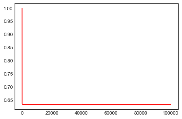
The probability rapidly drops to around $\frac{2}{3}$

x = np.arange(1, 10, 1)
y = 1 - (1 - 1/x)**x

plt.plot(x, y, color='r')

[<matplotlib.lines.Line2D at 0x121806ac8>]

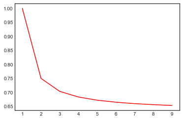
then slowly asymptotically approaches the limit

$\underset{n \rightarrow \infty}{\lim} 1 - (1 - \frac{1}{n})^n = 1 - e^{-1} \approx 0.6321$

h.

data = np.arange(1, 101, 1)

sum([4 in np.random.choice(data, size=100, replace=True) for i in range(10000)])/10000

0.6308

Very close to the expected value of

1 - (1 - 1/100)**100

0.6339676587267709

Exercise 3: $k$-fold Cross Validation

See section 5.1.3 in the notes

Exercise 4: Estimate the standard deviation of a predicted reponse

Suppose given $(X, Y)$ we predict $\hat{Y}$. This is an estimator [^0]. To estimate its standard error using data $(x_1, y_1), \dots, (x_n, y_n)$ use the “plug-in” estimator ¹.

$\hat{se}(\hat{Y}) = \sqrt{\frac{1}{n} \sum_{i = 1}^ n \left(\hat{y}_i - \overline{\hat{y}}\right)^2}$

where $\hat{y}_i$ is the predicted value for $x_i$ and $\overline{\hat{y}}$ is the mean predicted value.

In other words, use the sample standard deviation of the predicted values.

Footnotes