islr notes and exercises from An Introduction to Statistical Learning
4. Logistic Regression
Exercise 11: Classify high/low mpg cars in Auto dataset
Prepare the dataset
import pandas as pd

auto = pd.read_csv('http://www-bcf.usc.edu/~gareth/ISL/Auto.csv')
###
## impute missing horsepower values with mean
#

# replace `?` with 0 so means can be calculated
for index in auto.index:
    if auto.loc[index, 'horsepower'] == '?':
        auto.loc[index, 'horsepower'] = 0

# cast horsepower to numeric dtype
auto.loc[ : , 'horsepower'] = pd.to_numeric(auto.horsepower)

# now impute values
for index in auto.index:
    if auto.loc[index, 'horsepower'] == 0:
        auto.loc[index, 'horsepower'] = auto[auto.cylinders == auto.loc[index, 'cylinders']].horsepower.mean()
a. Create high and low mpg classes
# represent high mpg as mpg above the median
auto['mpg01'] = (auto.mpg > auto.mpg.median()).astype('int32')
auto.head()
| mpg | cylinders | displacement | horsepower | weight | acceleration | year | origin | name | mpg01 | |
|---|---|---|---|---|---|---|---|---|---|---|
| 0 | 18.0 | 8 | 307.0 | 130.0 | 3504 | 12.0 | 70 | 1 | chevrolet chevelle malibu | 0 |
| 1 | 15.0 | 8 | 350.0 | 165.0 | 3693 | 11.5 | 70 | 1 | buick skylark 320 | 0 |
| 2 | 18.0 | 8 | 318.0 | 150.0 | 3436 | 11.0 | 70 | 1 | plymouth satellite | 0 |
| 3 | 16.0 | 8 | 304.0 | 150.0 | 3433 | 12.0 | 70 | 1 | amc rebel sst | 0 |
| 4 | 17.0 | 8 | 302.0 | 140.0 | 3449 | 10.5 | 70 | 1 | ford torino | 0 |
auto.info()
<class 'pandas.core.frame.DataFrame'>
RangeIndex: 397 entries, 0 to 396
Data columns (total 10 columns):
mpg             397 non-null float64
cylinders       397 non-null int64
displacement    397 non-null float64
horsepower      397 non-null float64
weight          397 non-null int64
acceleration    397 non-null float64
year            397 non-null int64
origin          397 non-null int64
name            397 non-null object
mpg01           397 non-null int32
dtypes: float64(4), int32(1), int64(4), object(1)
memory usage: 29.5+ KB
Note high mpg is represented by class 1
b. Visual feature selection
import seaborn as sns
sns.set_style('white')

import warnings
warnings.filterwarnings('ignore')
Quantitative features
We’ll inspect some plots of the quantitative variables against the high/low classes first.
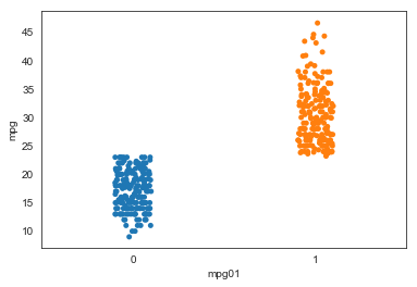
Of course, mpg will completely separate classes, which is unsurprising. We won’t use this feature in our models, since it seems like cheating and/or makes the exercise uninteresting.
ax = sns.stripplot(x="mpg01", y="mpg", data=auto)
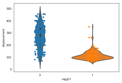
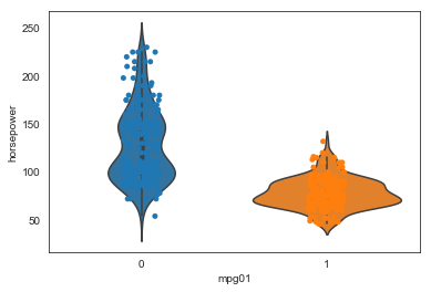
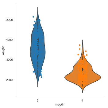
Now let’s look at the other quanitative features
ax = sns.violinplot(x="mpg01", y="displacement", data=auto)
ax = sns.stripplot(x="mpg01", y="displacement", data=auto)
ax = sns.violinplot(x="mpg01", y="horsepower", data=auto)
ax = sns.stripplot(x="mpg01", y="horsepower", data=auto)
ax = sns.catplot(x="mpg01", y="weight", data=auto, kind='violin')
ax = sns.stripplot(x="mpg01", y="weight", data=auto)
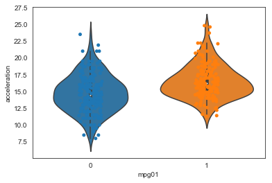
ax = sns.violinplot(x="mpg01", y="acceleration", data=auto)
ax = sns.stripplot(x="mpg01", y="acceleration", data=auto)
Since the number of unique values for year is small
auto.year.unique()
array([70, 71, 72, 73, 74, 75, 76, 77, 78, 79, 80, 81, 82])
one might argue it should be trasted as a qualitative variable. However, since there it has a natural (time) ordering we treat it as quantitative
ax = sns.catplot(x="mpg01", y="year", data=auto, kind='violin')
ax = sns.stripplot(x="mpg01", y="year", data=auto)
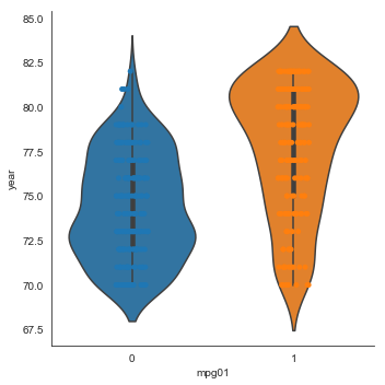
With the exception of acceleration and possibly year, all these plots show a good separation of the distributions across the mpg classes. Based on these plots, all the quantitative variable except acceleration look like useful features for predicting mpg class.
Qualitative features
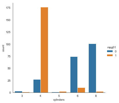
ax = sns.catplot(x="cylinders", hue='mpg01', data=auto, kind='count')
ax = sns.catplot(x="origin", hue='mpg01', data=auto, kind='count')
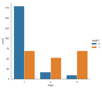
Since cylinders and origin separate the mpg classes well they both should be useful predictors.
Note: we’re going to ignore name for now. This is a categorical variable but it has a lot of levels
len(auto.name.unique())
304
and analysis is likely a bit complicated
c. Train-test split
import sklearn.model_selection as skl_model_selection
import statsmodels.api as sm
X, y = sm.add_constant(auto.drop(['acceleration', 'mpg01', 'name'], axis=1).values), auto.mpg01.values
X_train, X_test, y_train, y_test = skl_model_selection.train_test_split(X, y)
d. LDA model
import sklearn.discriminant_analysis as skl_discriminant_analysis

LDA_model = skl_discriminant_analysis.LinearDiscriminantAnalysis()
import sklearn.metrics as skl_metrics

skl_metrics.accuracy_score(y_test, LDA_model.fit(X_train, y_train).predict(X_test))
0.93
Impressive!
e. QDA model
QDA_model = skl_discriminant_analysis.QuadraticDiscriminantAnalysis()
skl_metrics.accuracy_score(y_test, QDA_model.fit(X_train, y_train).predict(X_test))
0.48
Much worse :(
f. Logit model
import sklearn.linear_model as skl_linear_model

Logit_model = skl_linear_model.LogisticRegression()
skl_metrics.accuracy_score(y_test, Logit_model.fit(X_train, y_train).predict(X_test))
0.94
Better!
g. KNN model
import sklearn.neighbors as skl_neighbors
models = {}
accuracies = {}

for i in range(1, 11):
    name = 'KNN' + str(i)
    models[name] = skl_neighbors.KNeighborsClassifier(n_neighbors=i)
    accuracies[name] = skl_metrics.accuracy_score(y_test, models[name].fit(X_train, y_train).predict(X_test))
pd.DataFrame(accuracies, index=[0]).sort_values(by=[0], axis='columns', ascending=False)
| KNN5 | KNN9 | KNN10 | KNN3 | KNN7 | KNN1 | KNN6 | KNN8 | KNN4 | KNN2 | |
|---|---|---|---|---|---|---|---|---|---|---|
| 0 | 0.83 | 0.83 | 0.83 | 0.82 | 0.82 | 0.8 | 0.8 | 0.8 | 0.76 | 0.7 |
These values are all really close, except perhaps . Given the bias-variance tradeoff, we’d probably want to select or based on these results