islr notes and exercises from An Introduction to Statistical Learning
4. Logistic Regression
Exercise 10: Classifying Direction in the Weekly dataset
- Preparing the Data
- a. Numerical and graphical summaries
- b. Logistic Regression Classification of
DirectionusingLagandVolumepredictors - c. Confusion Matrix
- d. Logistic Regression Classification of
DirectionusingLag2predictor - e. Other classification models of
DirectionusingLag2predictor - h. Which method has the best results?
- i. Feature and Model Selection
- Get all predictor interactions
- Choose some transformations
- Random data tweak
- Comparison of Logit, LDA, QDA, and KNN models on a single random data tweak
- <a href="#comparison-of-logit-lda-qda-and-knn-models-over--data-tweaks" data-toc-modified-id="Comparison-of-Logit,-LDA,-QDA,-and-KNN-models-over--data-tweaks-8.5">Comparison of Logit, LDA, QDA, and KNN models over data tweaks</a>
- Analysis of Comparisons
Preparing the Data
Import
import pandas as pd

weekly = pd.read_csv('../../datasets/Weekly.csv', index_col=0)
weekly.head()
| Year | Lag1 | Lag2 | Lag3 | Lag4 | Lag5 | Volume | Today | Direction | |
|---|---|---|---|---|---|---|---|---|---|
| 1 | 1990 | 0.816 | 1.572 | -3.936 | -0.229 | -3.484 | 0.154976 | -0.270 | Down |
| 2 | 1990 | -0.270 | 0.816 | 1.572 | -3.936 | -0.229 | 0.148574 | -2.576 | Down |
| 3 | 1990 | -2.576 | -0.270 | 0.816 | 1.572 | -3.936 | 0.159837 | 3.514 | Up |
| 4 | 1990 | 3.514 | -2.576 | -0.270 | 0.816 | 1.572 | 0.161630 | 0.712 | Up |
| 5 | 1990 | 0.712 | 3.514 | -2.576 | -0.270 | 0.816 | 0.153728 | 1.178 | Up |
weekly.info()
<class 'pandas.core.frame.DataFrame'>
Int64Index: 1089 entries, 1 to 1089
Data columns (total 9 columns):
Year         1089 non-null int64
Lag1         1089 non-null float64
Lag2         1089 non-null float64
Lag3         1089 non-null float64
Lag4         1089 non-null float64
Lag5         1089 non-null float64
Volume       1089 non-null float64
Today        1089 non-null float64
Direction    1089 non-null object
dtypes: float64(7), int64(1), object(1)
memory usage: 85.1+ KB
Preprocessing
Converting qualitative variables to quantitative
Don’t see any null values but let’s check
weekly.isna().sum().sum()
0
Direction is a qualitative variable encoded as a string; let’s encode it numerically
import sklearn.preprocessing as skl_preprocessing

# create and fit label encoder
direction_le = skl_preprocessing.LabelEncoder()
direction_le.fit(weekly.Direction)

# replace string encoding with numeric
weekly['Direction_num'] = direction_le.transform(weekly.Direction)
weekly.Direction_num.head()
1    0
2    0
3    1
4    1
5    1
Name: Direction_num, dtype: int64
direction_le.classes_
array(['Down', 'Up'], dtype=object)
direction_le.transform(direction_le.classes_)
array([0, 1])
So the encoding is {Down:0, Up:1}
a. Numerical and graphical summaries
Here’s a description of the dataset from the R documentation
Weekly S&P Stock Market Data

Description

Weekly percentage returns for the S&P 500 stock index between 1990 and 2010.

Usage

Weekly
Format

A data frame with 1089 observations on the following 9 variables.

Year
The year that the observation was recorded

Lag1
Percentage return for previous week

Lag2
Percentage return for 2 weeks previous

Lag3
Percentage return for 3 weeks previous

Lag4
Percentage return for 4 weeks previous

Lag5
Percentage return for 5 weeks previous

Volume
Volume of shares traded (average number of daily shares traded in billions)

Today
Percentage return for this week

Direction
A factor with levels Down and Up indicating whether the market had a positive or negative return on a given week

Source

Raw values of the S&P 500 were obtained from Yahoo Finance and then converted to percentages and lagged.
Let’s look at summary statistics
weekly.describe()
| Year | Lag1 | Lag2 | Lag3 | Lag4 | Lag5 | Volume | Today | Direction_num | |
|---|---|---|---|---|---|---|---|---|---|
| count | 1089.000000 | 1089.000000 | 1089.000000 | 1089.000000 | 1089.000000 | 1089.000000 | 1089.000000 | 1089.000000 | 1089.000000 |
| mean | 2000.048669 | 0.150585 | 0.151079 | 0.147205 | 0.145818 | 0.139893 | 1.574618 | 0.149899 | 0.555556 |
| std | 6.033182 | 2.357013 | 2.357254 | 2.360502 | 2.360279 | 2.361285 | 1.686636 | 2.356927 | 0.497132 |
| min | 1990.000000 | -18.195000 | -18.195000 | -18.195000 | -18.195000 | -18.195000 | 0.087465 | -18.195000 | 0.000000 |
| 25% | 1995.000000 | -1.154000 | -1.154000 | -1.158000 | -1.158000 | -1.166000 | 0.332022 | -1.154000 | 0.000000 |
| 50% | 2000.000000 | 0.241000 | 0.241000 | 0.241000 | 0.238000 | 0.234000 | 1.002680 | 0.241000 | 1.000000 |
| 75% | 2005.000000 | 1.405000 | 1.409000 | 1.409000 | 1.409000 | 1.405000 | 2.053727 | 1.405000 | 1.000000 |
| max | 2010.000000 | 12.026000 | 12.026000 | 12.026000 | 12.026000 | 12.026000 | 9.328214 | 12.026000 | 1.000000 |
-
All the variables ranges look good (e.g. no negative values for volume)
-
The
Lagvariables andTodayall have very similar summary statistics, as expected. -
Of particular interest is
Direction_num, which has a mean of and a standard deviation of ! That’s what we’ll be trying to predict later in the exercise, which will be interesting.
Let’s look at distributions
import seaborn as sns
import matplotlib.pyplot as plt
%matplotlib inline
plt.style.use('seaborn-white')
sns.set_style('white')

import warnings
warnings.filterwarnings('ignore')

import numpy as np
sns.pairplot(weekly, hue='Direction')
<seaborn.axisgrid.PairGrid at 0x1a2515d208>
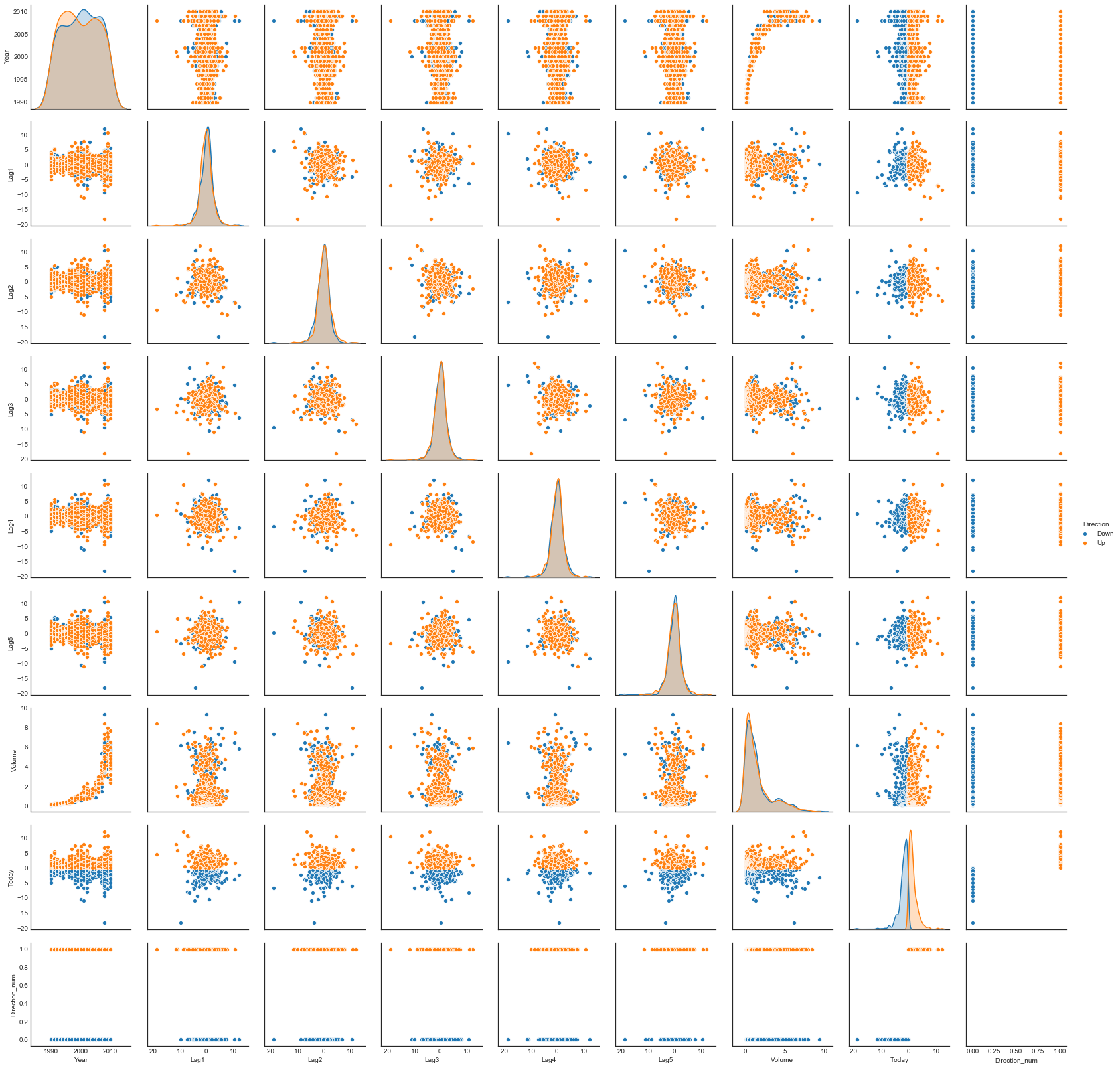
The return variables are concentrated
The return variables (i.e. Lag and Today variables) are “tight” instead of spread out, i.e. fairly concentrated about their mean.
Here are the deviations of all variables as percentages of the magnitude of their ranges
weekly_num = weekly.drop('Direction', axis=1)
round(100 * (weekly_num.std() / (weekly_num.max() - weekly_num.min())), 2)
Year             30.17
Lag1              7.80
Lag2              7.80
Lag3              7.81
Lag4              7.81
Lag5              7.81
Volume           18.25
Today             7.80
Direction_num    49.71
dtype: float64
Return variables are nearly uncorrelated
In the pairplot there is a visible lack of pairwise sample correlation among the return variables.
weekly.corr()
| Year | Lag1 | Lag2 | Lag3 | Lag4 | Lag5 | Volume | Today | Direction_num | |
|---|---|---|---|---|---|---|---|---|---|
| Year | 1.000000 | -0.032289 | -0.033390 | -0.030006 | -0.031128 | -0.030519 | 0.841942 | -0.032460 | -0.022200 |
| Lag1 | -0.032289 | 1.000000 | -0.074853 | 0.058636 | -0.071274 | -0.008183 | -0.064951 | -0.075032 | -0.050004 |
| Lag2 | -0.033390 | -0.074853 | 1.000000 | -0.075721 | 0.058382 | -0.072499 | -0.085513 | 0.059167 | 0.072696 |
| Lag3 | -0.030006 | 0.058636 | -0.075721 | 1.000000 | -0.075396 | 0.060657 | -0.069288 | -0.071244 | -0.022913 |
| Lag4 | -0.031128 | -0.071274 | 0.058382 | -0.075396 | 1.000000 | -0.075675 | -0.061075 | -0.007826 | -0.020549 |
| Lag5 | -0.030519 | -0.008183 | -0.072499 | 0.060657 | -0.075675 | 1.000000 | -0.058517 | 0.011013 | -0.018168 |
| Volume | 0.841942 | -0.064951 | -0.085513 | -0.069288 | -0.061075 | -0.058517 | 1.000000 | -0.033078 | -0.017995 |
| Today | -0.032460 | -0.075032 | 0.059167 | -0.071244 | -0.007826 | 0.011013 | -0.033078 | 1.000000 | 0.720025 |
| Direction_num | -0.022200 | -0.050004 | 0.072696 | -0.022913 | -0.020549 | -0.018168 | -0.017995 | 0.720025 | 1.000000 |
Indeed the magnitudes of the sample correlations for these pairs are quite small.
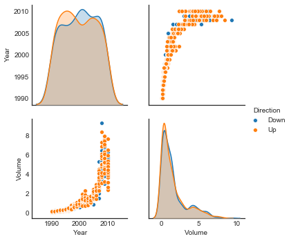
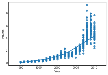
Volume correlates with Year
sns.pairplot(weekly, vars=['Year', 'Volume'], hue='Direction')
<seaborn.axisgrid.PairGrid at 0x1a28503780>
sns.regplot(weekly.Year, weekly.Volume, lowess=True)
<matplotlib.axes._subplots.AxesSubplot at 0x1a2a543be0>
b. Logistic Regression Classification of Direction using Lag and Volume predictors
import statsmodels.api as sm

# predictor labels
predictors = ['Lag' + stri. for i in range(1, 6)]
predictors += ['Volume']

# fit and summarize model

sm_logit_model_full = sm.Logit(weekly.Direction_num, sm.add_constant(weekly[predictors]))
sm_logit_model_full.fit().summary()
Optimization terminated successfully.
         Current function value: 0.682441
         Iterations 4
| Dep. Variable: | Direction_num | No. Observations: | 1089 |
|---|---|---|---|
| Model: | Logit | Df Residuals: | 1082 |
| Method: | MLE | Df Model: | 6 |
| Date: | Mon, 26 Nov 2018 | Pseudo R-squ.: | 0.006580 |
| Time: | 17:27:33 | Log-Likelihood: | -743.18 |
| converged: | True | LL-Null: | -748.10 |
| LLR p-value: | 0.1313 |
| coef | std err | z | P>|z| | [0.025 | 0.975] | |
|---|---|---|---|---|---|---|
| const | 0.2669 | 0.086 | 3.106 | 0.002 | 0.098 | 0.435 |
| Lag1 | -0.0413 | 0.026 | -1.563 | 0.118 | -0.093 | 0.010 |
| Lag2 | 0.0584 | 0.027 | 2.175 | 0.030 | 0.006 | 0.111 |
| Lag3 | -0.0161 | 0.027 | -0.602 | 0.547 | -0.068 | 0.036 |
| Lag4 | -0.0278 | 0.026 | -1.050 | 0.294 | -0.080 | 0.024 |
| Lag5 | -0.0145 | 0.026 | -0.549 | 0.583 | -0.066 | 0.037 |
| Volume | -0.0227 | 0.037 | -0.616 | 0.538 | -0.095 | 0.050 |
Only the intercept and Lag2 and appear to be statistically significant
c. Confusion Matrix
import sklearn.linear_model as skl_linear_model

# fit model
skl_logit_model_full = skl_linear_model.LogisticRegression()
X, Y = sm.add_constant(weekly[predictors]).values, weekly.Direction_num.values
skl_logit_model_full.fit(X, Y)
LogisticRegression(C=1.0, class_weight=None, dual=False, fit_intercept=True,
          intercept_scaling=1, max_iter=100, multi_class='warn',
          n_jobs=None, penalty='l2', random_state=None, solver='warn',
          tol=0.0001, verbose=0, warm_start=False)
# check paramaters are close in the two models
abs(skl_logit_model_full.coef_ - sm_logit_model_full.fit().params.values)
Optimization terminated successfully.
         Current function value: 0.682441
         Iterations 4


array([[1.33953314e-01, 6.15092984e-05, 3.94405141e-06, 4.06643634e-05,
        5.96004698e-05, 3.92562567e-05, 3.22507048e-04]])
import sklearn.metrics as skl_metrics

# confusion matrix
confusion_array = skl_metrics.confusion_matrix(Y, skl_logit_model_full.predict(X))
confusion_array
array([[ 54, 430],
       [ 47, 558]])
# confusion data frame
col_index = pd.MultiIndex.from_product([['Pred'], [0, 1]])
row_index = pd.MultiIndex.from_product([['Actual'], [0, 1]])
confusion_df = pd.DataFrame(confusion_array, columns=col_index, index=row_index)
confusion_df.loc[: ,('Pred','Total')] = confusion_df.Pred[0] + confusion_df.Pred[1]
confusion_df.loc[('Actual','Total'), :] = (confusion_df.loc[('Actual',0), :] +
                                        confusion_df.loc[('Actual',1), :])
confusion_df.astype('int32')
| Pred | ||||
|---|---|---|---|---|
| 0 | 1 | Total | ||
| Actual | 0 | 54 | 430 | 484 |
| 1 | 47 | 558 | 605 | |
| Total | 101 | 988 | 1089 | |
Performance rates of interest from the confusion matrix
Recall that for a binary classifier the confusion matrix shows
where
Also recall the following rates of interest
- The accuracy of the classifier is the proportion of correctly classified observations
i.e., “How often is the model right?”
- The misclassification rate (or error rate) is the proportion of incorrectly classified observations
i.e., “How often is the model wrong?”
- The null error rate is the proportion of the majority class
i.e. “How often would we be wrong if we always predicted the majority class”
- The true positive rate (or sensitivity or recall) is the ratio of true positives to actual positives
, “How often is the model right for actual positives ()?”
- The false positive rate is the ratio of false positives to actual negatives
i.e., “How often is the model wrong for actual positives?”
- The true negative rate or specificity is the ratio of true negatives to actual negatives
i.e., “How often is the model right for actual negatives ()?”
- The false negative rate is the ratio of true negatives to actual negatives
i.e., “How often is the model wrong for actual negatives ()?”
- The precision is the ratio of true positives to predicted positives
i.e., “How often are the models’ positive predictions right?”
- The prevalence is the ratio of actual positives to total observations
i.e., “How often do actual positives occur in the sample?”
Analyzing model performance rates
# necessary variables
n = confusion_df.loc[('Actual', 'Total'), ('Pred', 'Total')]
TN = confusion_df.loc[('Actual', 0), ('Pred', 0)]
FP = confusion_df.loc[('Actual', 0), ('Pred', 1)]
FN = confusion_df.loc[('Actual', 1), ('Pred', 0)]
TP = confusion_df.loc[('Actual', 1), ('Pred', 1)]

# compute rates
rates = {}
rates['accuracy'] = (TP + TN) / n
rates['error rate'] = (FP + FN) / n
rates['null error'] = max(FN + TP, FP + TN) / n
rates['TP rate'] = TP / (FN + TP)
rates['FP rate'] = FP / (FN + TP)
rates['TN rate'] = TN / (FP + TN)
rates['FN rate'] = FN / (FP + TN)
rates['precision'] = TP / (FP + TP)
rates['prevalence'] = (FN + TP) / n


# store results
model_perf_rates_df = pd.DataFrame(rates, index=[0])
model_perf_rates_df
| accuracy | error rate | null error | TP rate | FP rate | TN rate | FN rate | precision | prevalence | |
|---|---|---|---|---|---|---|---|---|---|
| 0 | 0.561983 | 0.438017 | 0.555556 | 0.922314 | 0.710744 | 0.11157 | 0.097107 | 0.564777 | 0.555556 |
Observations
-
The accuracy is so the model is right a bit more than half the time
-
The error rate is so the model is wrong a bit less than half the time
-
The “null error rate” is the error rate of the “null classifier” which always predicts the majority class, which in this case is . Thus our model is about as accurate as the null classifier.
-
The true positive and false positive rates are relatively high. The true negative and false negative rates are relatively low. This makes sense – inspection of the confusion matrix shows that the model predicts positives almost an order of magnitude more often
-
The precision is so the model correctly predicts positives a little more than half the time
-
The prevalence is also so positives occur in the sample a little more than half the time
We’ll package this functionality for later use:
def confusion_results(X, y, skl_model_fit):
    # get confusion array
    confusion_array = skl_metrics.confusion_matrix(y, skl_model_fit.predict(X))

    # necessary variables
    n = np.sum(confusion_array)
    TN = confusion_array[0, 0]
    FP = confusion_array[0, 1]
    FN = confusion_array[1, 0]
    TP = confusion_array[1, 1]

    # compute rates
    rates = {}
    rates['accuracy'] = (TP + TN) / n
    rates['error rate'] = (FP + FN) / n
    rates['null error'] = max(FN + TP, FP + TN) / n
    rates['TP rate'] = TP / (FN + TP)
    rates['FP rate'] = FP / (FN + TP)
    rates['TN rate'] = TN / (FP + TN)
    rates['FN rate'] = FN / (FP + TN)
    rates['precision'] = TP / (FP + TP)
    rates['prevalence'] = (FN + TP) / n


    # return results
    return pd.DataFrame(rates, index=[0])
confusion_results(X, Y, skl_logit_model_full.fit(X, Y))
| accuracy | error rate | null error | TP rate | FP rate | TN rate | FN rate | precision | prevalence | |
|---|---|---|---|---|---|---|---|---|---|
| 0 | 0.561983 | 0.438017 | 0.555556 | 0.922314 | 0.710744 | 0.11157 | 0.097107 | 0.564777 | 0.555556 |
d. Logistic Regression Classification of Direction using Lag2 predictor
In this section we do some feature selection. Since in b. we found that only Lag2 was a significant feature, we’ll eliminate the others. Further, we’ll train on the years 1990 to 2008 and test on 2009 to 2010
# train/test split
weekly_test, weekly_train = weekly[weekly['Year'] <= 2008], weekly[weekly['Year'] > 2008]
X_train, y_train = sm.add_constant(weekly_train['Lag2']), weekly_train['Direction_num']
X_test, y_test = sm.add_constant(weekly_test['Lag2']), weekly_test['Direction_num']

# fit new model
skl_logit_model_lag2 = skl_linear_model.LogisticRegression()
# confusion matrix
confusion_results(X_test, y_test, skl_logit_model_lag2.fit(X_train, y_train))
| accuracy | error rate | null error | TP rate | FP rate | TN rate | FN rate | precision | prevalence | |
|---|---|---|---|---|---|---|---|---|---|
| 0 | 0.550254 | 0.449746 | 0.552284 | 0.963235 | 0.777574 | 0.040816 | 0.045351 | 0.553326 | 0.552284 |
The accuracy is actually slightly worse than the full model
e. Other classification models of Direction using Lag2 predictor
LDA
import sklearn.discriminant_analysis as skl_discriminant_analysis

skl_LDA_model_lag2 = skl_discriminant_analysis.LinearDiscriminantAnalysis()
# confusion matrix
confusion_results(X_test, y_test, skl_LDA_model_lag2.fit(X_train, y_train))
| accuracy | error rate | null error | TP rate | FP rate | TN rate | FN rate | precision | prevalence | |
|---|---|---|---|---|---|---|---|---|---|
| 0 | 0.550254 | 0.449746 | 0.552284 | 0.965074 | 0.779412 | 0.038549 | 0.043084 | 0.553214 | 0.552284 |
# accuracy
skl_metrics.accuracy_score(y_test, skl_LDA_model_lag2.predict(X_test))
0.550253807106599
Nearly identical to skl_logit_model_lag2!
QDA
skl_QDA_model_lag2 = skl_discriminant_analysis.QuadraticDiscriminantAnalysis()
# confusion matrix
confusion_results(X_test, y_test, skl_QDA_model_lag2.fit(X_train, y_train))
| accuracy | error rate | null error | TP rate | FP rate | TN rate | FN rate | precision | prevalence | |
|---|---|---|---|---|---|---|---|---|---|
| 0 | 0.447716 | 0.552284 | 0.552284 | 0.0 | 0.0 | 1.0 | 1.23356 | NaN | 0.552284 |
Worse accuracy than Logistic Regression and LDA
KNN
import sklearn.neighbors as skl_neighbors

skl_KNN_model_lag2 = skl_neighbors.KNeighborsClassifier(n_neighbors=1)
# confusion matrix
confusion_results(X_test, y_test, skl_KNN_model_lag2.fit(X_train, y_train))
| accuracy | error rate | null error | TP rate | FP rate | TN rate | FN rate | precision | prevalence | |
|---|---|---|---|---|---|---|---|---|---|
| 0 | 0.518782 | 0.481218 | 0.552284 | 0.626838 | 0.498162 | 0.385488 | 0.460317 | 0.55719 | 0.552284 |
Comparing results
For neatness and ease of comparison, we’ll package all these results
def confusion_comparison(X, y, models):
    df = pd.concat([confusion_results(X, y, models[model_name])
                      for model_name in models])
    df['Model'] = list(models.keys())
    return df.set_index('Model')
models = {'Logit': skl_logit_model_lag2, 'LDA': skl_LDA_model_lag2,
          'QDA': skl_QDA_model_lag2, 'KNN': skl_KNN_model_lag2}
for model_name in models:
    models[model_name] = models[model_name].fit(X_train, y_train)

conf_comp_df = confusion_comparison(X_test, y_test, models)
conf_comp_df
| accuracy | error rate | null error | TP rate | FP rate | TN rate | FN rate | precision | prevalence | |
|---|---|---|---|---|---|---|---|---|---|
| Model | |||||||||
| Logit | 0.550254 | 0.449746 | 0.552284 | 0.963235 | 0.777574 | 0.040816 | 0.045351 | 0.553326 | 0.552284 |
| LDA | 0.550254 | 0.449746 | 0.552284 | 0.965074 | 0.779412 | 0.038549 | 0.043084 | 0.553214 | 0.552284 |
| QDA | 0.447716 | 0.552284 | 0.552284 | 0.000000 | 0.000000 | 1.000000 | 1.233560 | NaN | 0.552284 |
| KNN | 0.518782 | 0.481218 | 0.552284 | 0.626838 | 0.498162 | 0.385488 | 0.460317 | 0.557190 | 0.552284 |
h. Which method has the best results?
As measured by accuracy, Logit and LDA models are tied, with KNN not too far behind and QDA a more distant third.
With respect to other confusion metrics, Logit and LDA are nearly identical
i. Feature and Model Selection
In this section, we’ll experiment to try to find improved performance on the test data. We’ll try:
- Different subsets of the predictors
- Interactions among the predictors
- Transformations of the predictors
- Different values of for KNN
Get all predictor interactions
from itertools import combinations

# all pairs of columns in weekly except year and direction
df = weekly.drop(['Year', 'Direction', 'Direction_num'], axis=1)
col_pairs = combinations(df.columns, 2)

# assemble interactions in dataframe
interaction_df = pd.DataFrame({col1 + ':' + col2: weekly[col1]*weekly[col2]
                               for (col1, col2) in col_pairs})

# concat data frames
dir_df = weekly[['Direction', 'Direction_num']]
weekly_interact = pd.concat([weekly.drop(['Direction', 'Direction_num'], axis=1),
                             interaction_df, dir_df], axis=1)
weekly_interact.head()
| Year | Lag1 | Lag2 | Lag3 | Lag4 | Lag5 | Volume | Today | Lag1:Lag2 | Lag1:Lag3 | ... | Lag3:Volume | Lag3:Today | Lag4:Lag5 | Lag4:Volume | Lag4:Today | Lag5:Volume | Lag5:Today | Volume:Today | Direction | Direction_num | |
|---|---|---|---|---|---|---|---|---|---|---|---|---|---|---|---|---|---|---|---|---|---|
| 1 | 1990 | 0.816 | 1.572 | -3.936 | -0.229 | -3.484 | 0.154976 | -0.270 | 1.282752 | -3.211776 | ... | -0.609986 | 1.062720 | 0.797836 | -0.035490 | 0.061830 | -0.539936 | 0.940680 | -0.041844 | Down | 0 |
| 2 | 1990 | -0.270 | 0.816 | 1.572 | -3.936 | -0.229 | 0.148574 | -2.576 | -0.220320 | -0.424440 | ... | 0.233558 | -4.049472 | 0.901344 | -0.584787 | 10.139136 | -0.034023 | 0.589904 | -0.382727 | Down | 0 |
| 3 | 1990 | -2.576 | -0.270 | 0.816 | 1.572 | -3.936 | 0.159837 | 3.514 | 0.695520 | -2.102016 | ... | 0.130427 | 2.867424 | -6.187392 | 0.251265 | 5.524008 | -0.629120 | -13.831104 | 0.561669 | Up | 1 |
| 4 | 1990 | 3.514 | -2.576 | -0.270 | 0.816 | 1.572 | 0.161630 | 0.712 | -9.052064 | -0.948780 | ... | -0.043640 | -0.192240 | 1.282752 | 0.131890 | 0.580992 | 0.254082 | 1.119264 | 0.115081 | Up | 1 |
| 5 | 1990 | 0.712 | 3.514 | -2.576 | -0.270 | 0.816 | 0.153728 | 1.178 | 2.501968 | -1.834112 | ... | -0.396003 | -3.034528 | -0.220320 | -0.041507 | -0.318060 | 0.125442 | 0.961248 | 0.181092 | Up | 1 |
5 rows × 31 columns
Choose some transformations
# list of transformations

from numpy import sqrt, sin, log, exp, power

# power functions with odd exponent to preserve sign of inputs
def power_3(array):
    return np.power(array, 3)

def power_5(array):
    return np.power(array, 3)

def power_7(array):
    return np.power(array, 4)

# transformations are functions with domain all real numbers
transforms = [power_3, power_5, power_7, sin, exp]
transforms
[<function __main__.power_3(array)>,
 <function __main__.power_5(array)>,
 <function __main__.power_7(array)>,
 <ufunc 'sin'>,
 <ufunc 'exp'>]
Random data tweak
We’ll write a simple function which returns a dataset which has
- as predictors a random subset of the predictors and interactions of the original dataset (i.e. a random subset of the columns of
weekly_interact) - a random subset of its predictors transformed by a random choice of transformations from
transform
We call such a dataset a “random data tweak”
import numpy as np

def random_data_tweak(weekly_interact, transforms):
    # drop undersirable columns
    weekly_drop = weekly_interact.drop(['Year', 'Direction', 'Direction_num'], axis=1)

    # choose a random subset of the predictors
    predictor_labels = np.random.choice(weekly_drop.columns,
                                  size=np.random.randint(1, high=weekly_drop.shape[1] + 1),
                                  replace=False)


    # choose a random subset of these to transform
    trans_predictor_labels = np.random.choice(predictor_labels,
                                          size=np.random.randint(0, len(predictor_labels)),
                                          replace=False)

    # choose random transforms
    some_transforms = np.random.choice(transforms,
                                  size=len(trans_predictor_labels),
                                  replace=True)

    # create the df
    df = weekly_interact[predictor_labels].copy()

    # transform appropriate columns
    for i in range(0, len(trans_predictor_labels)):
        # do transformation
        df.loc[ : , trans_predictor_labels[i]] = some_transforms[i](df[trans_predictor_labels[i]])
        # rename to reflect which transformation was used
        df = df.rename({trans_predictor_labels[i]:
                    some_transforms[i].__name__ + '(' + trans_predictor_labels[i] + ')' }, axis='columns')

    return pd.concat([df, weekly_interact['Direction_num']], axis=1)
random_data_tweak(weekly_interact, transforms).head()
| Lag3-Lag5 | power_7(Volume-Today) | power_5(Lag5) | Lag2-Lag5 | power_3(Lag4-Lag5) | sin(Lag4) | Lag2-Today | exp(Lag1-Lag5) | Lag1 | power_5(Lag4-Volume) | exp(Lag1-Today) | Lag4-Today | sin(Lag5-Volume) | Lag3-Today | power_3(Lag3-Lag4) | exp(Lag2) | Direction_num | |
|---|---|---|---|---|---|---|---|---|---|---|---|---|---|---|---|---|---|
| 1 | 13.713024 | 0.000003 | -42.289684 | -5.476848 | 0.507856 | -0.227004 | -0.424440 | 0.058254 | 0.816 | -0.000045 | 0.802262 | 0.061830 | -0.514081 | 1.062720 | 0.732271 | 4.816271 | 0 |
| 2 | -0.359988 | 0.021456 | -0.012009 | -0.186864 | 0.732271 | 0.713448 | -2.102016 | 1.063781 | -0.270 | -0.199983 | 2.004751 | 10.139136 | -0.034017 | -4.049472 | -236.877000 | 2.261436 | 0 |
| 3 | -3.211776 | 0.099523 | -60.976890 | 1.062720 | -236.877000 | 0.999999 | -0.948780 | 25314.585232 | -2.576 | 0.015863 | 0.000117 | 5.524008 | -0.588434 | 2.867424 | 2.110708 | 0.763379 | 1 |
| 4 | -0.424440 | 0.000175 | 3.884701 | -4.049472 | 2.110708 | 0.728411 | -1.834112 | 250.637582 | 3.514 | 0.002294 | 12.206493 | 0.580992 | 0.251357 | -0.192240 | -0.010695 | 0.076078 | 1 |
| 5 | -2.102016 | 0.001075 | 0.543338 | 2.867424 | -0.010695 | -0.266731 | 4.139492 | 1.787811 | 0.712 | -0.000072 | 2.313441 | -0.318060 | 0.125113 | -3.034528 | 0.336456 | 33.582329 | 1 |
Comparison of Logit, LDA, QDA, and KNN models on a single random data tweak
import sklearn.model_selection as skl_model_selection

def model_comparison():
    # tweak data
    tweak_df = random_data_tweak(weekly_interact, transforms)

    # train test split
    X, y = sm.add_constant(tweak_df.drop(['Direction_num'], axis=1).values), tweak_df['Direction_num'].values
    X_train, X_test, y_train, y_test = skl_model_selection.train_test_split(X, y)

    # dict for models
    models = {}

    # train param models
    models['Logit'] = skl_linear_model.LogisticRegression(solver='lbfgs').fit(X_train, y_train)
    models['LDA'] = skl_discriminant_analysis.LinearDiscriminantAnalysis().fit(X_train, y_train)
    models['QDA'] =  skl_discriminant_analysis.QuadraticDiscriminantAnalysis().fit(X_train, y_train)

    # train KNN models for K = 1,..,5
    for i in range(1, 6):
        models['KNN' + stri.] = skl_neighbors.KNeighborsClassifier(n_neighbors=i).fit(X_train, y_train)


    return {'predictors': tweak_df.columns, 'comparison': confusion_comparison(X_test, y_test, models)}
model_comparison()
Comparison of Logit, LDA, QDA, and KNN models over data tweaks
def model_comparisons(n):
    # running list of predictors and dfs from each comparison
    predictors_list = []
    dfs = []

    # iterate comparisons
    for i in range(n):
        # get comparison result
        result = model_comparison()
        predictors_list += [result['predictors']]

        # set MultiIndex
        df = result['comparison']
        df['Instance'] = i
        df = df.reset_index()
        df  = df.set_index(['Instance', 'Model'])

        # add results to running lists
        dfs += [df]

    return {'predictors': predictors_list, 'comparisons': pd.concat(dfs)}
results = model_comparisons(1000)
Here are the first 3 comparisons:
comparisons_df = results['comparisons']
comparisons_df.head(21)
| accuracy | error rate | null error | TP rate | FP rate | TN rate | FN rate | precision | prevalence | ||
|---|---|---|---|---|---|---|---|---|---|---|
| Instance | Model | |||||||||
| 0 | Logit | 0.560440 | 0.439560 | 0.549451 | 0.666667 | 0.466667 | 0.430894 | 0.406504 | 0.588235 | 0.549451 |
| LDA | 0.948718 | 0.051282 | 0.549451 | 1.000000 | 0.093333 | 0.886179 | 0.000000 | 0.914634 | 0.549451 | |
| QDA | 0.450549 | 0.549451 | 0.549451 | 0.000000 | 0.000000 | 1.000000 | 1.219512 | NaN | 0.549451 | |
| KNN1 | 0.714286 | 0.285714 | 0.549451 | 0.760000 | 0.280000 | 0.658537 | 0.292683 | 0.730769 | 0.549451 | |
| KNN2 | 0.688645 | 0.311355 | 0.549451 | 0.553333 | 0.120000 | 0.853659 | 0.544715 | 0.821782 | 0.549451 | |
| KNN3 | 0.703297 | 0.296703 | 0.549451 | 0.740000 | 0.280000 | 0.658537 | 0.317073 | 0.725490 | 0.549451 | |
| KNN4 | 0.699634 | 0.300366 | 0.549451 | 0.653333 | 0.200000 | 0.756098 | 0.422764 | 0.765625 | 0.549451 | |
| KNN5 | 0.703297 | 0.296703 | 0.549451 | 0.760000 | 0.300000 | 0.634146 | 0.292683 | 0.716981 | 0.549451 | |
| 1 | Logit | 0.937729 | 0.062271 | 0.523810 | 0.979021 | 0.097902 | 0.892308 | 0.023077 | 0.909091 | 0.523810 |
| LDA | 0.695971 | 0.304029 | 0.523810 | 0.965035 | 0.545455 | 0.400000 | 0.038462 | 0.638889 | 0.523810 | |
| QDA | 0.476190 | 0.523810 | 0.523810 | 0.000000 | 0.000000 | 1.000000 | 1.100000 | NaN | 0.523810 | |
| KNN1 | 0.706960 | 0.293040 | 0.523810 | 0.769231 | 0.328671 | 0.638462 | 0.253846 | 0.700637 | 0.523810 | |
| KNN2 | 0.710623 | 0.289377 | 0.523810 | 0.587413 | 0.139860 | 0.846154 | 0.453846 | 0.807692 | 0.523810 | |
| KNN3 | 0.706960 | 0.293040 | 0.523810 | 0.790210 | 0.349650 | 0.615385 | 0.230769 | 0.693252 | 0.523810 | |
| KNN4 | 0.695971 | 0.304029 | 0.523810 | 0.650350 | 0.230769 | 0.746154 | 0.384615 | 0.738095 | 0.523810 | |
| KNN5 | 0.725275 | 0.274725 | 0.523810 | 0.825175 | 0.349650 | 0.615385 | 0.192308 | 0.702381 | 0.523810 | |
| 2 | Logit | 0.454212 | 0.545788 | 0.545788 | 0.000000 | 0.000000 | 1.000000 | 1.201613 | NaN | 0.545788 |
| LDA | 0.967033 | 0.032967 | 0.545788 | 0.959732 | 0.020134 | 0.975806 | 0.048387 | 0.979452 | 0.545788 | |
| QDA | 0.454212 | 0.545788 | 0.545788 | 0.000000 | 0.000000 | 1.000000 | 1.201613 | NaN | 0.545788 | |
| KNN1 | 0.501832 | 0.498168 | 0.545788 | 0.510067 | 0.422819 | 0.491935 | 0.588710 | 0.546763 | 0.545788 | |
| KNN2 | 0.487179 | 0.512821 | 0.545788 | 0.308725 | 0.248322 | 0.701613 | 0.830645 | 0.554217 | 0.545788 |
Here are the predictors used for the first 3 comparisons:
predictors_list = results['predictors']

predictors_list[0:3]
[Index(['Lag2-Today', 'Lag4-Volume', 'Lag2-Lag3', 'Volume-Today', 'Lag2',
        'power_7(Lag1-Volume)', 'Lag1-Lag2', 'Lag2-Volume', 'Lag4-Today',
        'sin(Lag3-Today)', 'Lag3-Lag4', 'Lag5-Volume', 'Today',
        'power_5(Lag3-Lag5)', 'Lag1-Lag5', 'Lag4', 'Direction_num'],
       dtype='object'),
 Index(['Lag3-Lag5', 'Lag5-Today', 'Lag1', 'sin(Lag2-Volume)', 'Lag2-Today',
        'power_5(Volume)', 'Lag4-Lag5', 'Lag1-Lag2', 'power_5(Lag2-Lag3)',
        'Lag3-Today', 'Lag3-Volume', 'Volume-Today', 'Lag1-Today',
        'Direction_num'],
       dtype='object'),
 Index(['power_3(Lag2-Lag3)', 'Lag1-Today', 'Lag4-Volume', 'sin(Lag1-Lag2)',
        'power_7(Lag2-Today)', 'Lag1', 'exp(Lag2-Lag4)', 'power_3(Volume)',
        'exp(Lag3-Lag5)', 'exp(Lag5)', 'power_5(Lag1-Lag5)', 'Today',
        'Lag1-Lag3', 'Lag4-Today', 'power_5(Lag5-Today)', 'exp(Lag3-Lag4)',
        'power_7(Lag3-Today)', 'sin(Lag2)', 'sin(Volume-Today)',
        'power_3(Lag2-Volume)', 'Lag1-Lag4', 'power_7(Lag4-Lag5)',
        'exp(Lag5-Volume)', 'Direction_num'],
       dtype='object')]
Analysis of Comparisons
Analyzing accuracy across models
Summary statistics
grouped_by_model = comparisons_df.groupby(level=1)
grouped_by_model.mean()
| accuracy | error rate | null error | TP rate | FP rate | TN rate | FN rate | precision | prevalence | |
|---|---|---|---|---|---|---|---|---|---|
| Model | |||||||||
| KNN1 | 0.626147 | 0.373853 | 0.556381 | 0.668314 | 0.342757 | 0.574424 | 0.418527 | 0.662625 | 0.55615 |
| KNN2 | 0.601912 | 0.398088 | 0.556381 | 0.463810 | 0.180901 | 0.775631 | 0.676137 | 0.707457 | 0.55615 |
| KNN3 | 0.629945 | 0.370055 | 0.556381 | 0.690867 | 0.358510 | 0.555069 | 0.390503 | 0.661137 | 0.55615 |
| KNN4 | 0.615769 | 0.384231 | 0.556381 | 0.544830 | 0.237261 | 0.705825 | 0.574505 | 0.691635 | 0.55615 |
| KNN5 | 0.631011 | 0.368989 | 0.556381 | 0.706117 | 0.371881 | 0.538619 | 0.371593 | 0.658446 | 0.55615 |
| LDA | 0.726355 | 0.273645 | 0.556381 | 0.942929 | 0.437290 | 0.456703 | 0.073307 | 0.717898 | 0.55615 |
| Logit | 0.551216 | 0.448784 | 0.556381 | 0.368049 | 0.176416 | 0.782584 | 0.797881 | 0.697051 | 0.55615 |
| QDA | 0.462040 | 0.537960 | 0.556381 | 0.085262 | 0.053065 | 0.933012 | 1.151742 | 0.619088 | 0.55615 |
grouped_by_model.mean().accuracy.sort_values(ascending=False)
Model
LDA      0.726355
KNN5     0.631011
KNN3     0.629945
KNN1     0.626147
KNN4     0.615769
KNN2     0.601912
Logit    0.551216
QDA      0.462040
Name: accuracy, dtype: float64
Let’s look at summary statistics for accuracy
grouped_by_model.accuracy.describe()
| count | mean | std | min | 25% | 50% | 75% | max | |
|---|---|---|---|---|---|---|---|---|
| Model | ||||||||
| KNN1 | 1000.0 | 0.626147 | 0.111154 | 0.435897 | 0.545788 | 0.600733 | 0.684982 | 1.000000 |
| KNN2 | 1000.0 | 0.601912 | 0.112694 | 0.421245 | 0.516484 | 0.578755 | 0.659341 | 1.000000 |
| KNN3 | 1000.0 | 0.629945 | 0.110973 | 0.443223 | 0.549451 | 0.604396 | 0.682234 | 1.000000 |
| KNN4 | 1000.0 | 0.615769 | 0.113840 | 0.410256 | 0.531136 | 0.589744 | 0.670330 | 0.996337 |
| KNN5 | 1000.0 | 0.631011 | 0.112222 | 0.439560 | 0.549451 | 0.600733 | 0.692308 | 1.000000 |
| LDA | 1000.0 | 0.726355 | 0.177813 | 0.476190 | 0.556777 | 0.699634 | 0.941392 | 0.996337 |
| Logit | 1000.0 | 0.551216 | 0.186576 | 0.369963 | 0.439560 | 0.468864 | 0.553114 | 1.000000 |
| QDA | 1000.0 | 0.462040 | 0.072413 | 0.369963 | 0.428571 | 0.446886 | 0.468864 | 0.967033 |
Interesting – all models were able to get very close to or achieve 100% accuracy at least once.
TO DO: Try to find similarities in predictors/transformations for the instances which gave maximum classification accuracy
Let’s look at some distributions.
Distributions of accuracy across models
Parametric models
import seaborn as sns
sns.set_style('white')

param_models = ['Logit', 'LDA', 'QDA']

for model_name in param_models:
    sns.distplot(grouped_by_model.accuracy.get_group(model_name), label=model_name)

plt.legend()
<matplotlib.legend.Legend at 0x1a254db860>
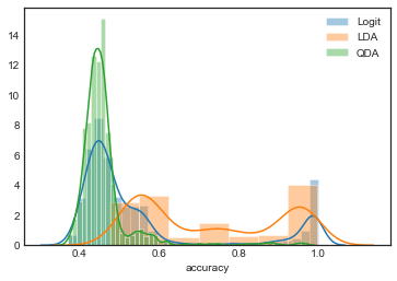
Observations
- There are some interesting peaks here – the distributions look bimodal.
- Both Logit and QDA models are highly concentrated in low accuracy, but LDA is more spread out
TO DO: Try to find similarities in predictors/transformations for the instances clustered around these two modes
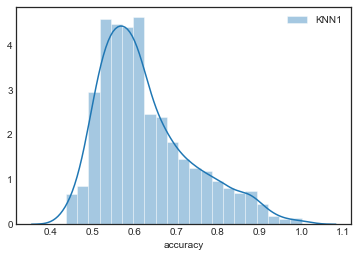
KNN models
sns.distplot(grouped_by_model.accuracy.get_group('KNN1'), label='KNN1')

plt.legend()
<matplotlib.legend.Legend at 0x1a252924a8>
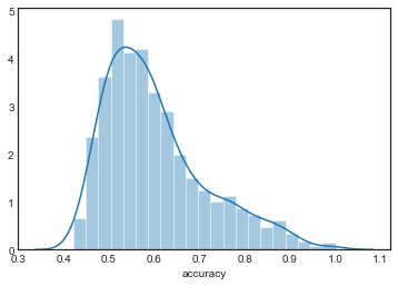
sns.distplot(grouped_by_model.accuracy.get_group('KNN2'), label='KNN2')
<matplotlib.axes._subplots.AxesSubplot at 0x1a2a6e6940>
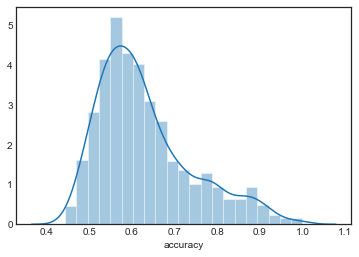
sns.distplot(grouped_by_model.accuracy.get_group('KNN3'), label='KNN3')
<matplotlib.axes._subplots.AxesSubplot at 0x1a25ce2cc0>
sns.distplot(grouped_by_model.accuracy.get_group('KNN4'), label='KNN4')
<matplotlib.axes._subplots.AxesSubplot at 0x1a2569ad30>
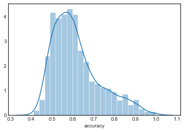
sns.distplot(grouped_by_model.accuracy.get_group('KNN5'), label='KNN5')
<matplotlib.axes._subplots.AxesSubplot at 0x1a25ca3dd8>
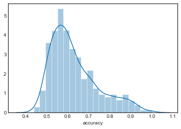
The distributions are all very similar, although they appear to become more concentrated as increases.