islr notes and exercises from An Introduction to Statistical Learning
3. Linear Regression
Exercise 14: The collinearity problem
- a. Generating the data
- b. Correlation among predictors
- c. Fitting a full OLS linear regression model
- d. Fitting an OLS linear regression model on the first predictor
- e. Fitting an OLS linear regression model on the second predictor
- f. Do these results contradict each other?
- g. Adding a mismeasured observation
a. Generating the data
In this problem the data are where and
- where
The regression coefficients are
import numpy as np
import pandas as pd

# set seed state for reproducibility
np.random.seed(0)

# generate data
x1 = np.random.uniform(size=100)
x2 = 0.5*x1 + np.random.normal(size=100)/100
y = 2 + 2*x1 + 0.3*x2

# collect data in dataframe
data = pd.DataFrame({'x1': x1, 'x2': x2, 'y':y})
data.head()
| x1 | x2 | y | |
|---|---|---|---|
| 0 | 0.548814 | 0.262755 | 3.176454 |
| 1 | 0.715189 | 0.366603 | 3.540360 |
| 2 | 0.602763 | 0.306038 | 3.297338 |
| 3 | 0.544883 | 0.257079 | 3.166890 |
| 4 | 0.423655 | 0.226710 | 2.915323 |
b. Correlation among predictors
The correlation matrix is
data.corr()
| x1 | x2 | y | |
|---|---|---|---|
| x1 | 1.000000 | 0.997614 | 0.999988 |
| x2 | 0.997614 | 1.000000 | 0.997936 |
| y | 0.999988 | 0.997936 | 1.000000 |
so the correlation among the predictors is approximately
round(data.corr().x1.x2, 3)
0.998
The scatterplot is
import seaborn as sns

sns.scatterplot(data.x1, data.x2)
<matplotlib.axes._subplots.AxesSubplot at 0x1a17257358>
c. Fitting a full OLS linear regression model
import statsmodels.formula.api as smf

full_model = smf.ols('y ~ x1 + x2', data=data).fit()
full_model.summary()
| Dep. Variable: | y | R-squared: | 1.000 |
|---|---|---|---|
| Model: | OLS | Adj. R-squared: | 1.000 |
| Method: | Least Squares | F-statistic: | 2.237e+30 |
| Date: | Sun, 11 Nov 2018 | Prob (F-statistic): | 0.00 |
| Time: | 14:03:46 | Log-Likelihood: | 3206.0 |
| No. Observations: | 100 | AIC: | -6406. |
| Df Residuals: | 97 | BIC: | -6398. |
| Df Model: | 2 | ||
| Covariance Type: | nonrobust |
| coef | std err | t | P>|t| | [0.025 | 0.975] | |
|---|---|---|---|---|---|---|
| Intercept | 2.0000 | 5.67e-16 | 3.53e+15 | 0.000 | 2.000 | 2.000 |
| x1 | 2.0000 | 1.47e-14 | 1.36e+14 | 0.000 | 2.000 | 2.000 |
| x2 | 0.3000 | 2.94e-14 | 1.02e+13 | 0.000 | 0.300 | 0.300 |
| Omnibus: | 4.521 | Durbin-Watson: | 0.105 |
|---|---|---|---|
| Prob(Omnibus): | 0.104 | Jarque-Bera (JB): | 3.208 |
| Skew: | -0.288 | Prob(JB): | 0.201 |
| Kurtosis: | 2.338 | Cond. No. | 128. |
Warnings:
[1] Standard Errors assume that the covariance matrix of the errors is correctly specified.
We find the estimators are
full_model.params
Intercept    2.0
x1           2.0
x2           0.3
dtype: float64
which is identical to .
The p-values for the estimators are
full_model.pvalues
Intercept    0.0
x1           0.0
x2           0.0
dtype: float64
So we can definitely reject the null hypotheses
d. Fitting an OLS linear regression model on the first predictor
x1_model = smf.ols('y ~ x1', data=data).fit()
x1_model.summary()
| Dep. Variable: | y | R-squared: | 1.000 |
|---|---|---|---|
| Model: | OLS | Adj. R-squared: | 1.000 |
| Method: | Least Squares | F-statistic: | 4.215e+06 |
| Date: | Sun, 11 Nov 2018 | Prob (F-statistic): | 7.26e-229 |
| Time: | 14:03:46 | Log-Likelihood: | 439.40 |
| No. Observations: | 100 | AIC: | -874.8 |
| Df Residuals: | 98 | BIC: | -869.6 |
| Df Model: | 1 | ||
| Covariance Type: | nonrobust |
| coef | std err | t | P>|t| | [0.025 | 0.975] | |
|---|---|---|---|---|---|---|
| Intercept | 2.0007 | 0.001 | 3450.157 | 0.000 | 2.000 | 2.002 |
| x1 | 2.1498 | 0.001 | 2052.992 | 0.000 | 2.148 | 2.152 |
| Omnibus: | 11.746 | Durbin-Watson: | 2.083 |
|---|---|---|---|
| Prob(Omnibus): | 0.003 | Jarque-Bera (JB): | 4.097 |
| Skew: | 0.138 | Prob(JB): | 0.129 |
| Kurtosis: | 2.047 | Cond. No. | 4.30 |
Warnings:
[1] Standard Errors assume that the covariance matrix of the errors is correctly specified.
In this case, but is a little off.
However, the p-value for are still zero, so we again reject the null hypothesis .
e. Fitting an OLS linear regression model on the second predictor
x2_model = smf.ols('y ~ x2', data=data).fit()
x2_model.summary()
| Dep. Variable: | y | R-squared: | 0.996 |
|---|---|---|---|
| Model: | OLS | Adj. R-squared: | 0.996 |
| Method: | Least Squares | F-statistic: | 2.366e+04 |
| Date: | Sun, 11 Nov 2018 | Prob (F-statistic): | 1.14e-118 |
| Time: | 14:03:46 | Log-Likelihood: | 180.49 |
| No. Observations: | 100 | AIC: | -357.0 |
| Df Residuals: | 98 | BIC: | -351.8 |
| Df Model: | 1 | ||
| Covariance Type: | nonrobust |
| coef | std err | t | P>|t| | [0.025 | 0.975] | |
|---|---|---|---|---|---|---|
| Intercept | 1.9957 | 0.008 | 257.091 | 0.000 | 1.980 | 2.011 |
| x2 | 4.2860 | 0.028 | 153.832 | 0.000 | 4.231 | 4.341 |
| Omnibus: | 12.365 | Durbin-Watson: | 2.101 |
|---|---|---|---|
| Prob(Omnibus): | 0.002 | Jarque-Bera (JB): | 4.200 |
| Skew: | -0.139 | Prob(JB): | 0.122 |
| Kurtosis: | 2.035 | Cond. No. | 7.33 |
Warnings:
[1] Standard Errors assume that the covariance matrix of the errors is correctly specified.
In this case, but is way off.
However, the p-value for are still zero, so we again reject the null hypothesis .
f. Do these results contradict each other?
Given that the authors want us to consider the correlation between the predictors, I think the intent of this question is to encourage us to wonder why, if are so strongly correlated, did the model do such a great job of estimating while the model did a poor job of estimating ?
It’s not clear how to answer this question.
g. Adding a mismeasured observation
First we add the new, mismeasured observation
new_row = pd.DataFrame({'x1': [0.1], 'x2': [0.8], 'y':[6]})
data = pd.concat([data, new_row]).reset_index()
data.tail()
| index | x1 | x2 | y | |
|---|---|---|---|---|
| 96 | 96 | 0.586513 | 0.285222 | 3.258593 |
| 97 | 97 | 0.020108 | 0.003158 | 2.041163 |
| 98 | 98 | 0.828940 | 0.409915 | 3.780854 |
| 99 | 99 | 0.004695 | 0.002523 | 2.010148 |
| 100 | 0 | 0.100000 | 0.800000 | 6.000000 |
Now we refit the models from c.-e..
full_model = smf.ols('y ~ x1 + x2', data=data).fit()
x1_model = smf.ols('y ~ x1', data=data).fit()
x2_model = smf.ols('y ~ x2', data=data).fit()
full_model.params
Intercept    1.991550
x1          -0.337428
x2           4.975187
dtype: float64
x1_model.params
Intercept    2.115685
x1           1.984495
dtype: float64
x2_model.params
Intercept    1.968755
x2           4.419615
dtype: float64
Now the paramter estimates of both the full model and -only model are off, while the -only model is pretty close.
full_model.pvalues
Intercept    1.926622e-133
x1            1.614723e-16
x2            4.878009e-90
dtype: float64
x1_model.pvalues
Intercept    3.830438e-51
x1           5.772966e-28
dtype: float64
x2_model.pvalues
Intercept    9.791075e-121
x2           3.652059e-102
dtype: float64
Both models are still really confident in rejecting the null hypothesis.
We’ll do a scatter plot to see if the new observation is an outlier.
import matplotlib.pyplot as plt
import seaborn as sns
from mpl_toolkits.mplot3d import Axes3D
%matplotlib inline
fig = plt.figure()
ax = Axes3D(fig)

ax.scatter(data['x1'], data['x2'], data['y'])
<mpl_toolkits.mplot3d.art3d.Path3DCollection at 0x1a24db2c50>
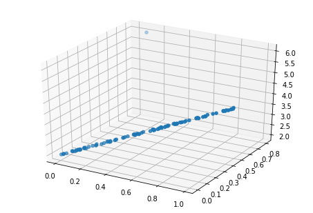
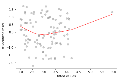
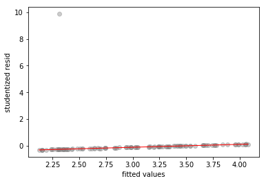
That new observation sure looks like an outlier. If we look at fitted-vs-residuals plots
# fitted-vs-residuals for the full model
sns.regplot(full_model.fittedvalues, full_model.resid/full_model.resid.std(),
            lowess=True,
            line_kws={'color':'r', 'lw':1},
            scatter_kws={'facecolors':'grey', 'edgecolors':'grey', 'alpha':0.4})
plt.xlabel('fitted values')
plt.ylabel('studentized resid')
Text(0,0.5,'studentized resid')
# fitted-vs-residuals for the X1 model
sns.regplot(x1_model.fittedvalues, x1_model.resid/x1_model.resid.std(),
            lowess=True,
            line_kws={'color':'r', 'lw':1},
            scatter_kws={'facecolors':'grey', 'edgecolors':'grey', 'alpha':0.4})
plt.xlabel('fitted values')
plt.ylabel('studentized resid')
Text(0,0.5,'studentized resid')
# fitted-vs-residuals for the X2 model
sns.regplot(x2_model.fittedvalues, x2_model.resid/x2_model.resid.std(),
            lowess=True,
            line_kws={'color':'r', 'lw':1},
            scatter_kws={'facecolors':'grey', 'edgecolors':'grey', 'alpha':0.4})
plt.xlabel('fitted values')
plt.ylabel('studentized resid')
Text(0,0.5,'studentized resid')
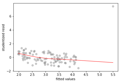
All three plots show a clear outlier. The -only and -only models also show high standardized residual values of and respectively, for the outlier.
Now we look at some leverage plots
# scatterplot of leverage vs studentized residuals
axes = sns.regplot(full_model.get_influence().hat_matrix_diag, full_model.resid/full_model.resid.std(),
            lowess=True,
            line_kws={'color':'r', 'lw':1},
            scatter_kws={'facecolors':'grey', 'edgecolors':'grey', 'alpha':0.4})
plt.xlabel('leverage')
plt.ylabel('studentized resid')

# plot Cook's distance contours for D = 0.5, D = 1
x = np.linspace(axes.get_xlim()[0], axes.get_xlim()[1], 50)
plt.plot(x, np.sqrt(0.5*(1 - x)/x), color='red', linestyle='dashed')
plt.plot(x, np.sqrt((1 - x)/x), color='red', linestyle='dashed')
/Users/home/anaconda3/lib/python3.6/site-packages/ipykernel_launcher.py:11: RuntimeWarning: invalid value encountered in sqrt
  # This is added back by InteractiveShellApp.init_path()
/Users/home/anaconda3/lib/python3.6/site-packages/ipykernel_launcher.py:12: RuntimeWarning: invalid value encountered in sqrt
  if sys.path[0] == '':


[<matplotlib.lines.Line2D at 0x1a264b3748>]
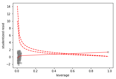
Since the mismeasured observation is has a Cook’s distance greater than 1, we’ll call it a high leverage point.