islr notes and exercises from An Introduction to Statistical Learning
3. Linear Regression
Exercise 13: Regression models on simulated data
- a. Generate feature data
- b. Generate noise
- c. Generate response data
- d. Scatterplot
- e. Fitting a least squares regression model
- f. Plotting the least squares and population lines
- g. Fitting a least squares quadratic regression model
- h. Repeating a. - f. with less noise
- i. Repeating a. - f. with more noise
- j. Confidence intervals for the coefficients
a. Generate feature data
import numpy as np

np.random.seed(0)
x = np.random.normal(loc=0, scale=1, size=100)
b. Generate noise
eps = np.random.normal(loc=0, scale=0.25, size=100)
c. Generate response data
y = -1 + 0.5*x + eps
y.shape
(100,)
In this case, .
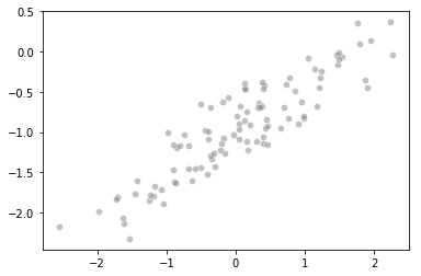
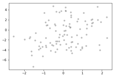
d. Scatterplot
%matplotlib inline
import seaborn as sns

sns.scatterplot(x, y, facecolors='grey', edgecolors='grey', alpha=0.5)
<matplotlib.axes._subplots.AxesSubplot at 0x1a201c7a58>
e. Fitting a least squares regression model
from sklearn.linear_model import LinearRegression

linear_model = LinearRegression().fit(x.reshape(-1, 1), y)
We find is
(round(linear_model.intercept_, 4), round(linear_model.coef_[0], 4))
(-0.9812, 0.5287)
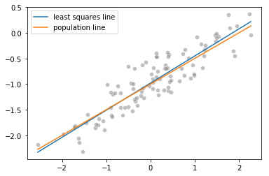
Not too far from the true value of (-1, 0.5)
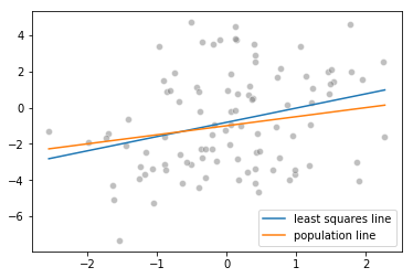
f. Plotting the least squares and population lines
import matplotlib.pyplot as plt

%matplotlib inline

sns.scatterplot(x, y, facecolors='grey', edgecolors='grey', alpha=0.5)
sns.lineplot(x, linear_model.predict(x.reshape(-1, 1)), label="least squares line")
sns.lineplot(x, -1 + 0.5*x, label="population line")

plt.legend()
<matplotlib.legend.Legend at 0x1a2019b550>
g. Fitting a least squares quadratic regression model
import pandas as pd

data_1 = pd.DataFrame({'x': x, 'x_sq': x**2, 'y': y})

quadratic_model = LinearRegression().fit(data_1[['x', 'x_sq']].values, data_1['y'].values)
In this case we find is
(round(quadratic_model.intercept_, 4), round(quadratic_model.coef_[0], 4))
(-0.9643, 0.5308)
The difference between the two models is
(round(abs(linear_model.intercept_ - quadratic_model.intercept_), 4),
 round(abs(linear_model.coef_[0] - quadratic_model.coef_[0]), 4))
(0.0169, 0.0021)
Still very close to the true value of (-1, 0.5), but not as close as the linear model. This at least is is not evidence that the quadratic term improves the fit
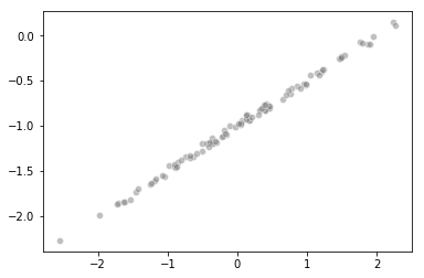
h. Repeating a. - f. with less noise
Generate feature data
import numpy as np

np.random.seed(0)
x = np.random.normal(loc=0, scale=1, size=100)
Generate noise with order of magnitude less variance
eps = np.random.normal(loc=0, scale=0.025, size=100)
Generate response data
y = -1 + 0.5*x + eps
y.shape
(100,)
Scatterplot
import seaborn as sns

sns.scatterplot(x, y, facecolors='grey', edgecolors='grey', alpha=0.5)
<matplotlib.axes._subplots.AxesSubplot at 0x1a20fadeb8>
Fitting a least squares regression model
from sklearn.linear_model import LinearRegression

linear_model = LinearRegression().fit(x.reshape(-1, 1), y)
We find is
(round(linear_model.intercept_, 4), round(linear_model.coef_[0], 4))
(-0.9981, 0.5029)
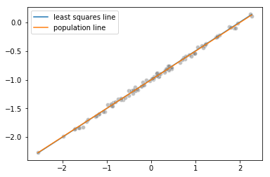
This is very close to the true value of (-1, 0.5)
Plotting the least squares and population lines
import matplotlib.pyplot as plt

%matplotlib inline

sns.scatterplot(x, y, facecolors='grey', edgecolors='grey', alpha=0.5)
sns.lineplot(x, linear_model.predict(x.reshape(-1, 1)), label="least squares line")
sns.lineplot(x, -1 + 0.5*x, label="population line")

plt.legend()
<matplotlib.legend.Legend at 0x1a20f06240>
Fitting a least squares quadratic regression model
import pandas as pd

data_2 = pd.DataFrame({'x': x, 'x_sq': x**2, 'y': y})

quadratic_model = LinearRegression().fit(data_2[['x', 'x_sq']].values, data_2['y'].values)
In this case we find is
(round(quadratic_model.intercept_, 4), round(quadratic_model.coef_[0], 4))
(-0.9964, 0.5031)
Still very close to the true value of (-1, 0.5), but not as close as the linear model.The difference between the two models is
(round(abs(linear_model.intercept_ - quadratic_model.intercept_), 4),
 round(abs(linear_model.coef_[0] - quadratic_model.coef_[0]), 4))
(0.0017, 0.0002)
However the difference between the two models is smaller now
i. Repeating a. - f. with more noise
Generate feature data
import numpy as np

np.random.seed(0)
x = np.random.normal(loc=0, scale=1, size=100)
Generate noise with order of magnitude more variance
eps = np.random.normal(loc=0, scale=2.5, size=100)
Generate response data
y = -1 + 0.5*x + eps
y.shape
(100,)
Scatterplot
import seaborn as sns

sns.scatterplot(x, y, facecolors='grey', edgecolors='grey', alpha=0.5)
<matplotlib.axes._subplots.AxesSubplot at 0x1a2114fbe0>
Fitting a least squares regression model
from sklearn.linear_model import LinearRegression

linear_model = LinearRegression().fit(x.reshape(-1, 1), y)
We find is
(round(linear_model.intercept_, 4), round(linear_model.coef_[0], 4))
(-0.8121, 0.7867)
Much farther from the true value of (-1, 0.5) in previous cases
Plotting the least squares and population lines
import matplotlib.pyplot as plt

%matplotlib inline

sns.scatterplot(x, y, facecolors='grey', edgecolors='grey', alpha=0.5)
sns.lineplot(x, linear_model.predict(x.reshape(-1, 1)), label="least squares line")
sns.lineplot(x, -1 + 0.5*x, label="population line")

plt.legend()
<matplotlib.legend.Legend at 0x1a21073748>
Fitting a least squares quadratic regression model
import pandas as pd

data_3 = pd.DataFrame({'x': x, 'x_sq': x**2, 'y': y})

quadratic_model = LinearRegression().fit(data_3[['x', 'x_sq']].values, data_3['y'].values)
In this case we find is
(round(quadratic_model.intercept_, 4), round(quadratic_model.coef_[0], 4))
(-0.6432, 0.8076)
Even further from the true value than the linear model
(round(abs(linear_model.intercept_ - quadratic_model.intercept_), 4),
 round(abs(linear_model.coef_[0] - quadratic_model.coef_[0]), 4))
(0.1689, 0.0208)
The difference between the two models is greater than the previous cases
j. Confidence intervals for the coefficients
import statsmodels.formula.api as smf

linear_model_1 = smf.ols('y ~ x', data=data_1).fit()
linear_model_2 = smf.ols('y ~ x', data=data_2).fit()
linear_model_3 = smf.ols('y ~ x', data=data_3).fit()
linear_model_1.conf_int()
| 0 | 1 | |
|---|---|---|
| Intercept | -1.03283 | -0.929593 |
| x | 0.47755 | 0.579800 |
linear_model_2.conf_int()
| 0 | 1 | |
|---|---|---|
| Intercept | -1.003283 | -0.992959 |
| x | 0.497755 | 0.507980 |
linear_model_3.conf_int()
| 0 | 1 | |
|---|---|---|
| Intercept | -1.328304 | -0.295930 |
| x | 0.275495 | 1.297997 |