3. Linear Regression

Exercise 10: Multiple regression of Sales on Price, Urban, and US features in Carseats dataset

Preparing the dataset

{

The Carseats dataset is part of the ISLR R package. We’ll use rpy2 to import ISLR into python

import numpy as np
import pandas as pd

carseats = pd.read_csv('../../datasets/Carseats.csv')

We’ll check for null entries

carseats.isna().sum().sum()

0

a. Fitting the model

Both Urban and US are binary class variables, so we can represent both by indicator variables (see section 3.3.1.

To encode the qualitative variables Urban and US, we’ll use a LabelEncoder from sklearn

from sklearn.preprocessing import LabelEncoder

# instantiate and encode labels
urban_le, us_le = LabelEncoder(), LabelEncoder()
urban_le.fit(carseats.Urban.unique())
us_le.fit(carseats.US.unique())

LabelEncoder()

urban_le.classes_

array(['No', 'Yes'], dtype=object)

Now we’ll create a dataframe with the qualitative variables numerically encoded

# copy
carseats_enc = carseats.copy()

# transform columns
carseats_enc.loc[ :, 'Urban'] = urban_le.transform(carseats['Urban'])
carseats_enc.loc[ :, 'US'] = us_le.transform(carseats['US'])

carseats_enc[['Urban', 'US']].head()

Now we can fit the model

import statsmodels.formula.api as smf

model = smf.ols('Sales ~ Urban + US + Price', data=carseats_enc).fit()
model.summary()

Warnings:
[1] Standard Errors assume that the covariance matrix of the errors is correctly specified.

b. Interpreting the coefficients

model.params

Intercept    13.043469
Urban        -0.021916
US            1.200573
Price        -0.054459
dtype: float64

Carseats has carseat sales data for 400 stores ¹

can interpret these coefficients as follows

1. The intercept $\hat{\beta}_0 = 13.04$ is the (estimated/predicted) average sales for carseats sold for free (Price=0) outside the US (US='No') and outside a city (Urban='No').
2. $\hat{\beta}_0 + \hat{\beta}_1 = 13.02$ is the estimated average sales for carseats sold in cities outside the US
3. $\hat{\beta}_0 + \hat{\beta}_2 = 14.24$ is the estimated average sales for carseats sold outside cities in the US
4. $\hat{\beta}_0 + \hat{\beta}_1 + \hat{\beta}_2 = 14.22$ is the estimated average sales for carseats sold in cities in the US
5. $\hat{\beta}_3 = -0.05$ so a $1 increase in price is estimated to decrease sales by $-0.05$

c. The formal model

Here we write the model in equation form. Let $X_1$ be Urban, $X_2$ be US, $X_3$ be Price. Then the model is

$Y = \beta_0 + \beta_1 X_1 + \beta_2 X_2 + \beta_3 X_3$

For the $i$-th observation, we have $\begin{aligned} y_i &= \beta_0 + \beta_1 x_{i1} + \beta_2 x_{i2} + \beta_3 x_{i3}\\ &= \begin{cases} \beta_0 + \beta_3 x_{i3} & \text{i-th carseat was sold outside a city, and outside the US}\\ \beta_0 + \beta_1 + \beta_3 x_{i3} & \text{i-th carseat was sold in a city outside the US}\\ \beta_0 + \beta_2 + \beta_3 x_{i3} & \text{i-th carseat was sold outside a city in the US}\\ \beta_0 + \beta_1 + \beta_2 + \beta_3 x_{i3} & \text{i-th carseat was sold in a US city}\\ \end{cases} \end{aligned}$

d. Significant Variables

is_stat_sig = model.pvalues < 0.05
model.pvalues[is_stat_sig]

Intercept    3.626602e-62
US           4.860245e-06
Price        1.609917e-22
dtype: float64

So we reject the null hypothesis $H_0: \beta_i = 0$ for $i=2, 3$, that is for the variables US and price.

model.pvalues[~ is_stat_sig]

Urban    0.935739
dtype: float64

We fail to reject the null hypothesis for $i=1$, that is for the variables Urban

e. Fitting a second model with price, US features

On the basis of d., we fit a new model with only the price and US variables

model_2 = smf.ols('Sales ~ US + Price', data=carseats_enc).fit()
model_2.summary()

Warnings:
[1] Standard Errors assume that the covariance matrix of the errors is correctly specified.

f. Goodness-of-fit for the two models

One way of determining how well the models fit the data is the $R^2$ values

print("The first model has R^2 = {}".format(round(model.rsquared, 3)))
print("The second model has R^2 = {}".format(round(model_2.rsquared, 3)))

The first model has R^2 = 0.239
The second model has R^2 = 0.239

So as far as the $R^2$ value is concerned, the models are equivalent. To choose one over the other, we might look at prediction accuracy, comparing mean squared errors, for example

print("The first model has model mean squared error {}".format(round(model.mse_model, 3)))
print("The first model has residual mean squared error {}".format(round(model.mse_resid, 3)))
print("The first model has total mean squared error {}".format(round(model.mse_total, 3)))

The first model has model mean squared error 253.813
The first model has residual mean squared error 6.113
The first model has total mean squared error 7.976

print("The second model has model mean squared error {}".format(round(model_2.mse_model, 3)))
print("The second model has residual mean squared error {}".format(round(model_2.mse_resid, 3)))
print("The second model has total mean squared error {}".format(round(model_2.mse_total, 3)))

The second model has model mean squared error 380.7
The second model has residual mean squared error 6.098
The second model has total mean squared error 7.976

print("The second model's model mse is {}% of the first".format(
      round(((model_2.mse_model - model.mse_model) * 100) / model.mse_model, 3)))
print("The second model's residual mse is {}% of the first".format(
      round(((model_2.mse_resid - model.mse_resid) * 100) / model.mse_resid, 3)))
print("The second model's total mse is {}% of the first".format(
      round(((model_2.mse_total - model.mse_total) * 100) / model.mse_total, 3)))

The second model's model mse is 49.992% of the first
The second model's residual mse is -0.25% of the first
The second model's total mse is 0.0% of the first

The statsmodel documentation has descriptions of these mean squared errors².

• The model mean squared error is “the explained sum of squares divided by the model degrees of freedom”
• The residual mean squared error is “the sum of squared residuals divided by the residual degrees of freedom”
• The total mean squared error is “the uncentered total sum of squares divided by n the number of observations”

In OLS multiple regression with $n$ observations and $p$ predictors, the number of model degrees of freedom are $p$, the number of residual degrees of freedom are $n - p - 1$, so we have

$\mathbf{mse}_{model} = \frac{1}{p}\left(\sum_{i = 1}^n (\hat{y}_i - \overline{y})^2\right)$ $\mathbf{mse}_{resid} = \frac{1}{n - p - 1}\left(\sum_{i = 1}^n (\hat{y}_i - y_i)^2\right)$ $\mathbf{mse}_{total} = \frac{1}{n}\left(\sum_{i = 1}^n (y_i - \overline{y})^2\right)$

From this we can draw some conclusions

• It’s clear why $\mathbf{mse}_{total}$ for the two models in this problem
• The error $\mathbf{mse}_{resid}$ is slightly smaller ($0.25\%$) for the second model, so it’s slightly at predicting the response.
• The error $\mathbf{mse}_{resid}$ is much larger ($50\%$) for the second model, so for this model the response predictions have a much greater deviation from average

From this perspective, the first model seems preferable, but it’s difficult to say. The tiebreaker should come from their performance on test data.

g. Confidence intervals for coefficients in the second model

model_2.conf_int()

h. Outliers and high leverage points in the second model

To check for outliers we look at a standardized residuals vs fitted values plot

import matplotlib.pyplot as plt
import seaborn as sns

%matplotlib inline

sns.regplot(model_2.get_prediction().summary_frame()['mean'], model_2.resid/model_2.resid.std(),
            lowess=True,
            line_kws={'color':'r', 'lw':1},
            scatter_kws={'facecolors':'grey', 'edgecolors':'grey', 'alpha':0.4})
plt.xlabel('fitted values')
plt.ylabel('studentized resid')

Text(0,0.5,'studentized resid')

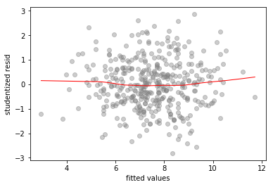
No outliers – all the studentized residual values are in the interval

((model_2.resid/model_2.resid.std()).min(), (model_2.resid/model_2.resid.std()).max())

(-2.812135116227541, 2.8627420897506766)

To check for high influence points we do an influence plot

# scatterplot of leverage vs studentized residuals
axes = sns.regplot(model_2.get_influence().hat_matrix_diag, model_2.resid/model_2.resid.std(), 
            lowess=True, 
            line_kws={'color':'r', 'lw':1},
            scatter_kws={'facecolors':'grey', 'edgecolors':'grey', 'alpha':0.4})
plt.xlabel('leverage')
plt.ylabel('studentized resid')

# plot Cook's distance contours for D = 0.5, D = 1
x = np.linspace(axes.get_xlim()[0], axes.get_xlim()[1], 50)
plt.plot(x, np.sqrt(0.5*(1 - x)/x), color='red', linestyle='dashed')
plt.plot(x, np.sqrt((1 - x)/x), color='red', linestyle='dashed')

[<matplotlib.lines.Line2D at 0x1a181ff6a0>]

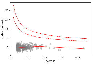
No high influence points. There is one rather high leverage point, but it has a low residual.

Footnotes