islr notes and exercises from An Introduction to Statistical Learning
3. Linear Regression
Exercise 9: Multiple regression of mpg on numerical features in auto
Preparing the dataset
Import pandas, load the Auto dataset, and inspect
import numpy as np
import pandas as pd

auto = pd.read_csv('../../datasets/Auto.csv')
auto.head()
| Unnamed: 0 | mpg | cylinders | displacement | horsepower | weight | acceleration | year | origin | name | |
|---|---|---|---|---|---|---|---|---|---|---|
| 0 | 1 | 18.0 | 8 | 307.0 | 130 | 3504 | 12.0 | 70 | 1 | chevrolet chevelle malibu |
| 1 | 2 | 15.0 | 8 | 350.0 | 165 | 3693 | 11.5 | 70 | 1 | buick skylark 320 |
| 2 | 3 | 18.0 | 8 | 318.0 | 150 | 3436 | 11.0 | 70 | 1 | plymouth satellite |
| 3 | 4 | 16.0 | 8 | 304.0 | 150 | 3433 | 12.0 | 70 | 1 | amc rebel sst |
| 4 | 5 | 17.0 | 8 | 302.0 | 140 | 3449 | 10.5 | 70 | 1 | ford torino |
auto.info()
<class 'pandas.core.frame.DataFrame'>
RangeIndex: 392 entries, 0 to 391
Data columns (total 10 columns):
Unnamed: 0      392 non-null int64
mpg             392 non-null float64
cylinders       392 non-null int64
displacement    392 non-null float64
horsepower      392 non-null int64
weight          392 non-null int64
acceleration    392 non-null float64
year            392 non-null int64
origin          392 non-null int64
name            392 non-null object
dtypes: float64(3), int64(6), object(1)
memory usage: 30.7+ KB
There are missing values represented by '?' in horsepower. We’ll impute these by using mean values for the cylinders class
# replace `?` with nans
auto.loc[:, 'horsepower'].apply(lambda x: np.nan if x == '?' else x)

# cast horsepower to numeric dtype
auto.loc[:, 'horsepower'] = pd.to_numeric(auto.horsepower)

# now impute values
auto.loc[:, 'horsepower'] = auto.horsepower.fillna(auto.horsepower.mean())
auto.info()
<class 'pandas.core.frame.DataFrame'>
RangeIndex: 392 entries, 0 to 391
Data columns (total 10 columns):
Unnamed: 0      392 non-null int64
mpg             392 non-null float64
cylinders       392 non-null int64
displacement    392 non-null float64
horsepower      392 non-null int64
weight          392 non-null int64
acceleration    392 non-null float64
year            392 non-null int64
origin          392 non-null int64
name            392 non-null object
dtypes: float64(3), int64(6), object(1)
memory usage: 30.7+ KB
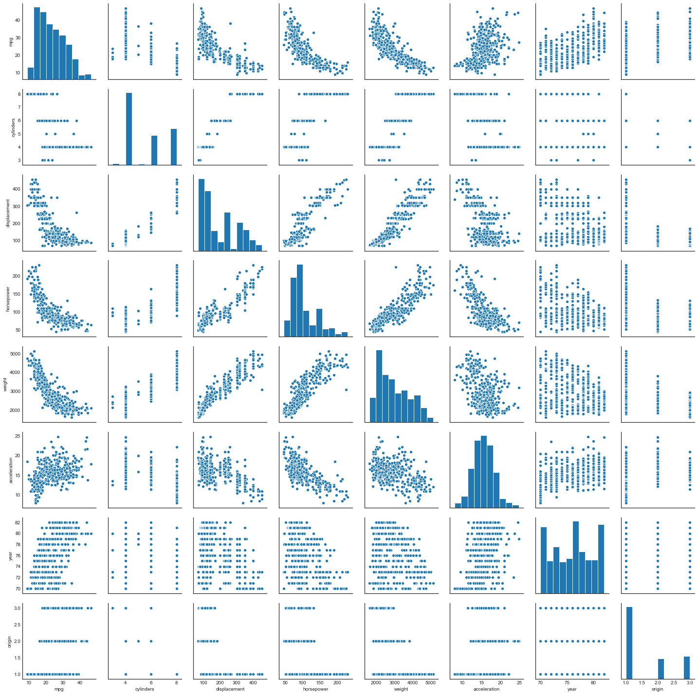
a. Scatterplot matrix of auto
# setup
import matplotlib.pyplot as plt
import seaborn as sns

%matplotlib inline
plt.style.use('seaborn-white')
sns.set_style('white')
sns.pairplot(auto.dropna())
b. Correlation matrix of auto
Compute the correlation matrix of the numerical variables
auto.corr()
| mpg | cylinders | displacement | horsepower | weight | acceleration | year | origin | |
|---|---|---|---|---|---|---|---|---|
| mpg | 1.000000 | -0.776260 | -0.804443 | -0.776230 | -0.831739 | 0.422297 | 0.581469 | 0.563698 |
| cylinders | -0.776260 | 1.000000 | 0.950920 | 0.843640 | 0.897017 | -0.504061 | -0.346717 | -0.564972 |
| displacement | -0.804443 | 0.950920 | 1.000000 | 0.897584 | 0.933104 | -0.544162 | -0.369804 | -0.610664 |
| horsepower | -0.776230 | 0.843640 | 0.897584 | 1.000000 | 0.864320 | -0.688223 | -0.415617 | -0.451925 |
| weight | -0.831739 | 0.897017 | 0.933104 | 0.864320 | 1.000000 | -0.419502 | -0.307900 | -0.581265 |
| acceleration | 0.422297 | -0.504061 | -0.544162 | -0.688223 | -0.419502 | 1.000000 | 0.282901 | 0.210084 |
| year | 0.581469 | -0.346717 | -0.369804 | -0.415617 | -0.307900 | 0.282901 | 1.000000 | 0.184314 |
| origin | 0.563698 | -0.564972 | -0.610664 | -0.451925 | -0.581265 | 0.210084 | 0.184314 | 1.000000 |
c. Fitting the model
import statsmodels.api as sm

# drop non-numerical columns and rows with null entries
model_df = auto.drop(['name'], axis=1).dropna()
X, Y = model_df.drop(['mpg'], axis=1), model_df.mpg

# add constant
X = sm.add_constant(X)

# create and fit model
model = sm.OLS(Y, X).fit()

# show results summary
model.summary()
| Dep. Variable: | mpg | R-squared: | 0.822 |
|---|---|---|---|
| Model: | OLS | Adj. R-squared: | 0.819 |
| Method: | Least Squares | F-statistic: | 256.4 |
| Date: | Sun, 28 Oct 2018 | Prob (F-statistic): | 1.89e-141 |
| Time: | 19:28:06 | Log-Likelihood: | -1037.2 |
| No. Observations: | 397 | AIC: | 2090. |
| Df Residuals: | 389 | BIC: | 2122. |
| Df Model: | 7 | ||
| Covariance Type: | nonrobust |
| coef | std err | t | P>|t| | [0.025 | 0.975] | |
|---|---|---|---|---|---|---|
| const | -18.0900 | 4.629 | -3.908 | 0.000 | -27.191 | -8.989 |
| cylinders | -0.4560 | 0.322 | -1.414 | 0.158 | -1.090 | 0.178 |
| displacement | 0.0196 | 0.008 | 2.608 | 0.009 | 0.005 | 0.034 |
| horsepower | -0.0136 | 0.014 | -0.993 | 0.321 | -0.040 | 0.013 |
| weight | -0.0066 | 0.001 | -10.304 | 0.000 | -0.008 | -0.005 |
| acceleration | 0.0998 | 0.098 | 1.021 | 0.308 | -0.092 | 0.292 |
| year | 0.7587 | 0.051 | 14.969 | 0.000 | 0.659 | 0.858 |
| origin | 1.4199 | 0.277 | 5.132 | 0.000 | 0.876 | 1.964 |
| Omnibus: | 30.088 | Durbin-Watson: | 1.294 |
|---|---|---|---|
| Prob(Omnibus): | 0.000 | Jarque-Bera (JB): | 48.301 |
| Skew: | 0.511 | Prob(JB): | 3.25e-11 |
| Kurtosis: | 4.370 | Cond. No. | 8.58e+04 |
Warnings:
[1] Standard Errors assume that the covariance matrix of the errors is correctly specified.
[2] The condition number is large, 8.58e+04. This might indicate that there are
strong multicollinearity or other numerical problems.
i. Is there a relationship between the predictors and the mpg?
This question is answered by the -value of the -statistic
model.f_pvalue
1.8936359873496686e-141
This is effectively zero, so the answer is yes
ii. Which predictors appear to have a statistically significant relationship to the response?
This is answered by the -values of the individual predictors
model.pvalues
const           1.097017e-04
cylinders       1.580259e-01
displacement    9.455004e-03
horsepower      3.212038e-01
weight          3.578587e-22
acceleration    3.077592e-01
year            2.502539e-40
origin          4.530034e-07
dtype: float64
A common cutoff is a -value of 0.05, so by this standard, the predictors with a statistically significant relationship to mpg are
is_stat_sig = model.pvalues < 0.05
model.pvalues[is_stat_sig]
const           1.097017e-04
displacement    9.455004e-03
weight          3.578587e-22
year            2.502539e-40
origin          4.530034e-07
dtype: float64
And those which do not are
model.pvalues[~ is_stat_sig]
cylinders       0.158026
horsepower      0.321204
acceleration    0.307759
dtype: float64
This is surprising, since we found a statistically significant relationship between horsepower and mpg in exercise 8.
iii. What does the coefficient for the year variable suggest?
That fuel efficiency has been improving over time
d. Diagnostic plots
First we assemble the results in a dataframe and clean up a bit
# get full prediction results
pred_df = model.get_prediction().summary_frame()

# rename columns to avoid `mean` name conflicts and other confusions
new_names = {}
for name in pred_df.columns:
    if 'mean' in name:
        new_names[name] = name.replace('mean', 'mpg_pred')
    elif 'obs_ci' in name:
        new_names[name] = name.replace('obs_ci', 'mpg_pred_pi')
    else:
        new_names[name] = name
pred_df = pred_df.rename(new_names, axis='columns')

# concat into final df
model_df = pd.concat([model_df, pred_df], axis=1)
model_df.head()
| mpg | cylinders | displacement | horsepower | weight | acceleration | year | origin | mpg_pred | mpg_pred_se | mpg_pred_ci_lower | mpg_pred_ci_upper | mpg_pred_pi_lower | mpg_pred_pi_upper | |
|---|---|---|---|---|---|---|---|---|---|---|---|---|---|---|
| 0 | 18.0 | 8 | 307.0 | 130.0 | 3504 | 12.0 | 70 | 1 | 14.966498 | 0.506952 | 13.969789 | 15.963208 | 8.338758 | 21.594239 |
| 1 | 15.0 | 8 | 350.0 | 165.0 | 3693 | 11.5 | 70 | 1 | 14.028743 | 0.446127 | 13.151621 | 14.905865 | 7.417930 | 20.639557 |
| 2 | 18.0 | 8 | 318.0 | 150.0 | 3436 | 11.0 | 70 | 1 | 15.262507 | 0.487309 | 14.304418 | 16.220595 | 8.640464 | 21.884549 |
| 3 | 16.0 | 8 | 304.0 | 150.0 | 3433 | 12.0 | 70 | 1 | 15.107684 | 0.493468 | 14.137487 | 16.077882 | 8.483879 | 21.731490 |
| 4 | 17.0 | 8 | 302.0 | 140.0 | 3449 | 10.5 | 70 | 1 | 14.948273 | 0.535264 | 13.895900 | 16.000646 | 8.311933 | 21.584612 |
Now we plot the 4 diagnostic plots returned by R’s lm() function (see [exercise 8)
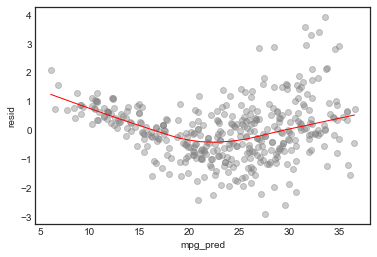
Standardized residuals vs fitted value
# add residuals to df
model_df['resid'] = model.resid


# plot
plt.ylabel('standardized resid')
sns.regplot(model_df.mpg_pred, model_df.resid/model_df.resid.std(), lowess=True,
            line_kws={'color':'r', 'lw':1},
            scatter_kws={'facecolors':'grey', 'edgecolors':'grey', 'alpha':0.4})
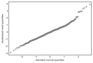
Standardized residuals QQ-plot
sm.qqplot(model_df.resid/model_df.resid.std(), color='grey', alpha=0.5, xlabel='')
plt.ylabel('studentized resid quantiles')
plt.xlabel('standard normal quantiles')
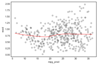
Scale-location plot
plt.ylabel('√|standardized resid|')
sns.regplot(model_df.mpg_pred, np.sqrt(np.abs(model_df.resid/model_df.resid.std())), lowess=True,
            line_kws={'color':'r', 'lw':1},
            scatter_kws={'facecolors':'grey', 'edgecolors':'grey', 'alpha':0.4})
Influence Plot
# influence plot
axes = sns.regplot(model.get_influence().hat_matrix_diag, model_df.resid/model_df.resid.std(),
            lowess=True,
            line_kws={'color':'r', 'lw':1},
            scatter_kws={'facecolors':'grey', 'edgecolors':'grey', 'alpha':0.4})
plt.xlabel('leverage')
plt.ylabel('studentized resid')
x = np.linspace(0.01, axes.get_xlim()[1], 50)
plt.plot(x, np.sqrt(0.5*(1 - x)/x), color='red', linestyle='dashed')
plt.plot(x, np.sqrt((1 - x)/x), color='red', linestyle='dashed')
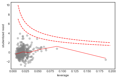
From these diagnostic plots we conclude
- There is non-linearity in the data
- There are a handful of outliers (studentized residual 3)
- The normality assumption is appropriate
- The data shows heteroscedasticity
- There are no high influence points
e. Interaction effects
We are told to use the * and ~ R operators to investigate interaction effects. Thankfully statmodels has support for these.
To use :
, we will fit a model consisting of only pairwise interaction terms
import itertools as it
import statsmodels.formula.api as smf


# generate formula for interaction terms
names = list(auto.columns.drop('name').drop('mpg'))
pairs = list(it.product(names, names))
terms  = [name1 + ' : ' + name2 for (name1, name2) in pairs if name1 != name2]
formula = 'mpg ~ '

for term in terms:
    formula += term + ' + '
formula = formula[:-3]
formula
'mpg ~ cylinders : displacement + cylinders : horsepower + cylinders : weight + cylinders : acceleration + cylinders : year + cylinders : origin + displacement : cylinders + displacement : horsepower + displacement : weight + displacement : acceleration + displacement : year + displacement : origin + horsepower : cylinders + horsepower : displacement + horsepower : weight + horsepower : acceleration + horsepower : year + horsepower : origin + weight : cylinders + weight : displacement + weight : horsepower + weight : acceleration + weight : year + weight : origin + acceleration : cylinders + acceleration : displacement + acceleration : horsepower + acceleration : weight + acceleration : year + acceleration : origin + year : cylinders + year : displacement + year : horsepower + year : weight + year : acceleration + year : origin + origin : cylinders + origin : displacement + origin : horsepower + origin : weight + origin : acceleration + origin : year'
# fit a regression model with only interaction terms
pair_int_model = smf.ols(formula=formula, data=auto).fit()
And find the statisitcally significant interactions
# show interactions with p value less than 0.05
pair_int_model.pvalues[pair_int_model.pvalues < 5e-2]
Intercept                    0.005821
cylinders:year               0.014595
displacement:acceleration    0.010101
displacement:year            0.000036
displacement:origin          0.015855
weight:acceleration          0.005177
acceleration:year            0.000007
year:origin                  0.045881
dtype: float64
Now to use + we fit a model consisting of all features and all possible interactions
# generate formula for interaction terms
names = list(auto.columns.drop('name').drop('mpg'))
formula = 'mpg ~ '
for name in names:
    formula += name + '*'
formula = formula[:-1]
formula
'mpg ~ cylinders*displacement*horsepower*weight*acceleration*year*origin'
# fit a regression model with all features and all possible interaction terms
full_int_model = smf.ols(formula=formula, data=auto).fit()
Finally, we find the statistically significant terms
full_int_model.pvalues[full_int_model.pvalues < 0.05]
Series([], dtype: float64)
In this case, including all possible interactions has led to none of them being statistically significant, even the pairwise interactions.
f. Variable transformations
We’ll try the suggested variable transformations .
# drop constant before transformation, else const for log(X) will be zero
X = X.drop('const', axis=1)
import numpy as np
import statsmodels.api as sm

# transform data
log_X = np.log(X)
sqrt_X = np.sqrt(X)
X_sq = X**2

# fit models with constants
log_model = sm.OLS(Y, sm.add_constant(log_X)).fit()
sqrt_model = sm.OLS(Y, sm.add_constant(sqrt_X)).fit()
sq_model = sm.OLS(Y, sm.add_constant(X_sq)).fit()
Now we’ll look at each of these models individually:
The log model
log_model.summary()
| Dep. Variable: | mpg | R-squared: | 0.848 |
|---|---|---|---|
| Model: | OLS | Adj. R-squared: | 0.845 |
| Method: | Least Squares | F-statistic: | 310.3 |
| Date: | Sun, 28 Oct 2018 | Prob (F-statistic): | 6.92e-155 |
| Time: | 19:28:07 | Log-Likelihood: | -1005.5 |
| No. Observations: | 397 | AIC: | 2027. |
| Df Residuals: | 389 | BIC: | 2059. |
| Df Model: | 7 | ||
| Covariance Type: | nonrobust |
| coef | std err | t | P>|t| | [0.025 | 0.975] | |
|---|---|---|---|---|---|---|
| const | -67.0838 | 17.433 | -3.848 | 0.000 | -101.358 | -32.810 |
| cylinders | 1.8114 | 1.658 | 1.093 | 0.275 | -1.448 | 5.070 |
| displacement | -1.0935 | 1.540 | -0.710 | 0.478 | -4.121 | 1.934 |
| horsepower | -6.2631 | 1.528 | -4.100 | 0.000 | -9.267 | -3.259 |
| weight | -13.4966 | 2.185 | -6.178 | 0.000 | -17.792 | -9.201 |
| acceleration | -4.3687 | 1.577 | -2.770 | 0.006 | -7.469 | -1.268 |
| year | 55.5963 | 3.540 | 15.704 | 0.000 | 48.636 | 62.557 |
| origin | 1.5763 | 0.506 | 3.118 | 0.002 | 0.582 | 2.570 |
| Omnibus: | 39.413 | Durbin-Watson: | 1.381 |
|---|---|---|---|
| Prob(Omnibus): | 0.000 | Jarque-Bera (JB): | 76.214 |
| Skew: | 0.576 | Prob(JB): | 2.82e-17 |
| Kurtosis: | 4.812 | Cond. No. | 1.36e+03 |
Warnings:
[1] Standard Errors assume that the covariance matrix of the errors is correctly specified.
[2] The condition number is large, 1.36e+03. This might indicate that there are
strong multicollinearity or other numerical problems.
Very large and very low -value for the -statistic suggest this is a useful model. Interestingly, this model gives very large -values for the features cylinders and displacement.
The statistically significant features of the the original and log models and their p-values
stat_sig_df = pd.concat([model.pvalues[is_stat_sig], log_model.pvalues[is_stat_sig]], join='outer', axis=1, sort=False)
stat_sig_df = stat_sig_df.rename({0 : 'model_pval', 1: 'log_model_pval'}, axis='columns')
stat_sig_df
| model_pval | log_model_pval | |
|---|---|---|
| const | 1.097017e-04 | 1.390585e-04 |
| displacement | 9.455004e-03 | 4.780250e-01 |
| weight | 3.578587e-22 | 1.641584e-09 |
| year | 2.502539e-40 | 2.150054e-43 |
| origin | 4.530034e-07 | 1.958604e-03 |
The insignificant features and p-values are
stat_sig_df = pd.concat([model.pvalues[~ is_stat_sig], log_model.pvalues[~ is_stat_sig]], join='outer', axis=1, sort=False)
stat_sig_df = stat_sig_df.rename({0 : 'model_pval', 1: 'log_model_pval'}, axis='columns')
stat_sig_df
| model_pval | log_model_pval | |
|---|---|---|
| cylinders | 0.158026 | 0.275162 |
| horsepower | 0.321204 | 0.000050 |
| acceleration | 0.307759 | 0.005869 |
So the original and log models are in total agreement about which features are significant!
Let’s look at prediction accuracy.
from sklearn.linear_model import LinearRegression
from sklearn.model_selection import train_test_split
from sklearn.metrics import mean_squared_error

# split the data
X_train, X_test, y_train, y_test = train_test_split(auto.drop(['name', 'mpg'], axis=1).dropna(), auto.mpg)

# transform
log_X_train, log_X_test = np.log(X_train), np.log(X_test)

# train models
reg_model = LinearRegression().fit(X_train, y_train)
log_model = LinearRegression().fit(log_X_train, y_train)

# get train mean squared errors
reg_train_mse = mean_squared_error(y_train, reg_model.predict(X_train))
log_train_mse = mean_squared_error(y_train, log_model.predict(log_X_train))

print("The reg model train mse is {} and the log model train mse is {}".format(round(reg_train_mse, 3), round(log_train_mse, 3)))

# get test mean squared errors
reg_test_mse = mean_squared_error(y_test, reg_model.predict(X_test))
log_test_mse = mean_squared_error(y_test, log_model.predict(log_X_test))

print("The reg model test mse is {} and the log model test mse is {}".format(round(reg_test_mse, 3), round(log_test_mse, 3)))
The reg model train mse is 11.111 and the log model train mse is 9.496
The reg model test mse is 10.434 and the log model test mse is 8.83
From a prediction standpoint, the model is an improvement
The square root model
sqrt_model.summary()
| Dep. Variable: | mpg | R-squared: | 0.834 |
|---|---|---|---|
| Model: | OLS | Adj. R-squared: | 0.831 |
| Method: | Least Squares | F-statistic: | 279.5 |
| Date: | Sun, 28 Oct 2018 | Prob (F-statistic): | 1.76e-147 |
| Time: | 19:29:40 | Log-Likelihood: | -1023.0 |
| No. Observations: | 397 | AIC: | 2062. |
| Df Residuals: | 389 | BIC: | 2094. |
| Df Model: | 7 | ||
| Covariance Type: | nonrobust |
| coef | std err | t | P>|t| | [0.025 | 0.975] | |
|---|---|---|---|---|---|---|
| const | -51.9765 | 9.138 | -5.688 | 0.000 | -69.942 | -34.011 |
| cylinders | -0.0144 | 1.535 | -0.009 | 0.993 | -3.031 | 3.003 |
| displacement | 0.2176 | 0.229 | 0.948 | 0.344 | -0.234 | 0.669 |
| horsepower | -0.6775 | 0.303 | -2.233 | 0.026 | -1.274 | -0.081 |
| weight | -0.6471 | 0.078 | -8.323 | 0.000 | -0.800 | -0.494 |
| acceleration | -0.5983 | 0.821 | -0.729 | 0.467 | -2.212 | 1.016 |
| year | 12.9347 | 0.854 | 15.139 | 0.000 | 11.255 | 14.614 |
| origin | 3.2448 | 0.763 | 4.253 | 0.000 | 1.745 | 4.745 |
| Omnibus: | 38.601 | Durbin-Watson: | 1.306 |
|---|---|---|---|
| Prob(Omnibus): | 0.000 | Jarque-Bera (JB): | 69.511 |
| Skew: | 0.589 | Prob(JB): | 8.05e-16 |
| Kurtosis: | 4.677 | Cond. No. | 3.30e+03 |
Warnings:
[1] Standard Errors assume that the covariance matrix of the errors is correctly specified.
[2] The condition number is large, 3.3e+03. This might indicate that there are
strong multicollinearity or other numerical problems.
The value is slightly less than for the log model, but not much, and the F-statistic p-value is comparable.
This model doesn’t like cylinder and displacement just like the regular and log models, but also rejects acceleration.
Now we’ll check prediction accuracy
# transform
sqrt_X_train, sqrt_X_test = np.sqrt(X_train), np.sqrt(X_test)

# train sqrt model
sqrt_model = LinearRegression().fit(sqrt_X_train, y_train)

# get train mean squared errors
reg_train_mse = mean_squared_error(y_train, reg_model.predict(X_train))
sqrt_train_mse = mean_squared_error(y_train, sqrt_model.predict(sqrt_X_train))

print("The reg model train mse is {} and the sqrt model train mse is {}".format(round(reg_train_mse, 3), round(sqrt_train_mse, 3)))

# get test mean squared errors
reg_test_mse = mean_squared_error(y_test, reg_model.predict(X_test))
sqrt_test_mse = mean_squared_error(y_test, sqrt_model.predict(sqrt_X_test))

print("The reg model test mse is {} and the sqrt model test mse is {}".format(round(reg_test_mse, 3), round(sqrt_test_mse, 3)))
The reg model train mse is 11.111 and the sqrt model train mse is 10.365
The reg model test mse is 10.434 and the sqrt model test mse is 9.635
Again, the model is better at prediction
The squared model
sq_model.summary()
| Dep. Variable: | mpg | R-squared: | 0.798 |
|---|---|---|---|
| Model: | OLS | Adj. R-squared: | 0.794 |
| Method: | Least Squares | F-statistic: | 219.3 |
| Date: | Sun, 28 Oct 2018 | Prob (F-statistic): | 8.35e-131 |
| Time: | 19:38:32 | Log-Likelihood: | -1062.3 |
| No. Observations: | 397 | AIC: | 2141. |
| Df Residuals: | 389 | BIC: | 2172. |
| Df Model: | 7 | ||
| Covariance Type: | nonrobust |
| coef | std err | t | P>|t| | [0.025 | 0.975] | |
|---|---|---|---|---|---|---|
| const | 0.9215 | 2.352 | 0.392 | 0.695 | -3.702 | 5.546 |
| cylinders | -0.0864 | 0.025 | -3.431 | 0.001 | -0.136 | -0.037 |
| displacement | 5.672e-05 | 1.39e-05 | 4.092 | 0.000 | 2.95e-05 | 8.4e-05 |
| horsepower | -2.945e-05 | 4.98e-05 | -0.591 | 0.555 | -0.000 | 6.85e-05 |
| weight | -9.535e-07 | 8.95e-08 | -10.653 | 0.000 | -1.13e-06 | -7.77e-07 |
| acceleration | 0.0066 | 0.003 | 2.466 | 0.014 | 0.001 | 0.012 |
| year | 0.0050 | 0.000 | 14.360 | 0.000 | 0.004 | 0.006 |
| origin | 0.4110 | 0.069 | 5.956 | 0.000 | 0.275 | 0.547 |
| Omnibus: | 20.163 | Durbin-Watson: | 1.296 |
|---|---|---|---|
| Prob(Omnibus): | 0.000 | Jarque-Bera (JB): | 27.033 |
| Skew: | 0.421 | Prob(JB): | 1.35e-06 |
| Kurtosis: | 3.961 | Cond. No. | 1.45e+08 |
Warnings:
[1] Standard Errors assume that the covariance matrix of the errors is correctly specified.
[2] The condition number is large, 1.45e+08. This might indicate that there are
strong multicollinearity or other numerical problems.
Slightly lower and higher -statistic -value than previous, but seems negligible (in all cases the -statistic -value is effectively zero)
Let’s check prediction accuracy
# transform
X_sq_train, X_sq_test = X_train**2, X_test**2

# train sqrt model
sq_model = LinearRegression().fit(X_sq_train, y_train)

# get train mean squared errors
reg_train_mse = mean_squared_error(y_train, reg_model.predict(X_train))
sq_train_mse = mean_squared_error(y_train, sq_model.predict(X_sq_train))

print("The reg model train mse is {} and the sq model train mse is {}".format(round(reg_train_mse, 3), round(sq_train_mse, 3)))

# get test mean squared errors
reg_test_mse = mean_squared_error(y_test, reg_model.predict(X_test))
sq_test_mse = mean_squared_error(y_test, sq_model.predict(sq_X_test))

print("The reg model test mse is {} and the sq model test mse is {}".format(round(reg_test_mse, 3), round(sq_test_mse, 3)))
The reg model train mse is 11.111 and the sq model train mse is 12.571
The reg model test mse is 10.434 and the sq model test mse is 12.0
So the model is not as good at predicting as any of the other models