3. Linear Regression

Conceptual Exercises

Exercise 1: Hypothesis testing the coefficients from the model in 3.2.1

Table 3.4 has the following information

import pandas as pd

data = {'Coefficient': [2.939, 0.046, 0.189, -0.001],
        'Std. Error': [0.3119, 0.0014, 0.0086, 0.0059],
        't-statistic': [9.42, 32.81, 21.89, -0.18],
        'p-value': [0.0001, 0.0001, 0.0001, 0.8599]}
index = ['Intercept', 'TV', 'radio', 'newspaper']
table = pd.DataFrame(data, index=index)
table.head()

The p-values for Intercept, TV and radio coefficients are small enough to reject the null hypotheses for these coefficient, thus accepting the alternative hypotheses that

• In the absence of TV and radio ad spending there will be 2,939 units sold
• For each $1,000 increase in TV ad spending another 46 units will sell
• For each $1,000 increase in radio ad spending another 189 units will sell

The p-value for newspaper is very high, so in that case we retain the null hypothesis that there is no relationship between newspaper ad spending and sales

Exercise 2: Differences between KNN classifier and regression methods

Both methods look at a neighborhood $N_0$ of the $K$ points nearest a point $x_0$.

The KNN classifier estimates the conditional probability of of a class $j$ based on the fraction of observations in the neighborhood of $x_0$ such that are in class $j$. It then predicts $y_0$ to be the class that maximizes this probability (using Bayes rule). Thus, the KNN classifier predicts a qualitative response (a discrete finite RV)

The KNN regression method, however, predicts the response value $y_0$ based on the average response value $\overline{y}$ of all observations in the neighborhood $N_0$. Thus, KNN regression predicts a quantitative response (a continuous RV).

Exercise 3: Regressing Salary on GPA, IQ, and Gender

We have predictors

$\begin{aligned} X_1 &= GPA\\ X_2 &= IQ\\ X_3 &= Gender\\ X_4 &= X_1X_2\\ X_5 &= X_1X_3 \end{aligned}$

And response

$Y = Salary$

where Salary means salary after graduation in units of $1,000.

Ordinary least squares (OLS) gives the estimated coefficients

$\begin{aligned} \hat{\beta}_0 &= 50\\ \hat{\beta}_1 &= 20\\ \hat{\beta}_2 &= 0.07\\ \hat{\beta}_3 &= 35\\ \hat{\beta}_4 &= 0.01\\ \hat{\beta}_5 &= -10 \end{aligned}$

a.

For a fixed value of IQ and GPA, $X_1, X_2$ are fixed and $X_3$ is variable. In this case we can write the model

$\hat{Y} = a + b X_3$

where we have absorbed the fixed values into

$\begin{aligned} a &= \beta_0 + \beta_1 X_1 + \beta_2 X_2 + \beta_4 X_1X_2\\ b &= \beta_3 + \beta_5 X_1 \end{aligned}$

For simplicity, assume values of 3.0 for GPA and 110 for IQ. Then we find

a = 50 + 20*3.0 + 0.07*110 + 0.01*3.0*110
b = 35 + -10*3.0
a, b

(121.0, 5.0)

So for the $i$-th person, the model predicts

$\hat{y}_i = 121 + 5x_{i3}$

and since $X_3$ is an indicator variable, the model predicts a salary of

$\hat{y}_i = \begin{cases} 126 &= \text{i-th person is female}\\ 121 &= \text{i-th person is female} \end{cases}$

so for a fixed $GPA$ and $IQ$, (answer ii) is correct.

NB: The actual values for salary here depended on our assumed values for IQ and GPA.

b.

a = 50 + 20*4.0 + 0.07*110 + 0.01*4.0*110
b = 35 + -10*4.0
print("The predicted salary for a female with an IQ of 110 and a GPA of 4.0 is ${} thousand".format(a + b))

The predicted salary for a female with an IQ of 110 and a GPA of 4.0 is $137.1 thousand

c.

The magnitude of a coefficient describes the magnitude of the effect, but not the evidence for it, which comes from the p-value of the hypothesis test for the coefficient. It’s possible to have a large coefficient but weak evidence (large p-value) and conversely a small coefficient but strong evidence (small p-value).

So as stated, the answer here is false (that is, it’s false as a conditional statement).

Exercise 4: Linear Vs. Non-linear Train and Test RSS

a.

If by “expect” we mean, averaged over many datasets, then the answer is that the linear model should have a lower train RSS.

b.

Same answer as a.

c.

If the true relationship is non-linear but unknown, then we don’t have enough information to say. For example the relationship could be “close to linear” (e.g. quadratic with extremely small $X^2$ coefficient, or piecewise linear) in which case on average we would expect better performance from the linear model. Or it could be polynomial of degree 3 or greater, in which case we’d expect the cubic model to perform better.

Testing my answers

In this section, I’m going to use simulation to test my answers.

# setup
import numpy as np
import pandas as pd
import statsmodels.formula.api as smf
from tqdm import tqdm_notebook

# generate coefficients for random linear function
def random_true_linear():
    coeffs = 20e3 * np.random.random_sample((2,)) - 10e3
    def f(x):
        return coeffs[1] + coeffs[0] * x
    return f

# generate n data points according to linear relationship
def gen_data(n_sample, true_f):
    # initialize df with uniformly random input
    df = pd.DataFrame({'x': 20e3 * np.random.random_sample((n_sample,)) - 10e3})
    # add linear outputs and noise
    df['y'] = df['x'].map(true_f) + np.random.normal(size=n_sample)**3
    # return df
    return df

# get test and train RSS from linear and cubic models from random linear function
def test_run(n_sample):
    # random linear function
    true_linear = random_true_linear()

    # generate train and test data
    train, test = gen_data(n_sample, true_linear), gen_data(n_sample, true_linear)

    # fit models
    linear_model = smf.ols('y ~ x', data=train).fit()
    cubic_model = smf.ols('y ~ x + I(x**2) + I(x**3)', data=train).fit()

    # get train RSSes
    linear_train_RSS, cubic_train_RSS = (linear_model.resid**2).sum(), (cubic_model.resid**2).sum()

    # get test RSSes
    linear_test_RSS = ((linear_model.predict(exog=test['x']) - test['y'])**2).sum()
    cubic_test_RSS =  ((cubic_model.predict(exog=test['x']) - test['y'])**2).sum()

    # create df and add test and train RSS
    df = pd.DataFrame(columns=pd.MultiIndex.from_product([['linear', 'cubic'], ['train', 'test']]))
    df.loc[0] = np.array([linear_train_RSS, linear_test_RSS, cubic_test_RSS, cubic_train_RSS])

    return df

# sample size, number of tests
n_sample, n_tests = 100, 1000

# dataframe for results
results = pd.DataFrame(columns=pd.MultiIndex.from_product([['linear', 'cubic'], ['train', 'test']]))

# iterate
for i in tqdm_notebook(range(n_tests)):
    results = results.append(test_run(n_sample), ignore_index=True)

results.head()

import matplotlib.pyplot as plt
import seaborn as sns

%matplotlib inline

plt.figure(figsize=(10,10))
plt.subplot(2, 1, 1)
sns.distplot(results.linear.train, label="Linear train RSS")
sns.distplot(results.linear.test, label="Linear test RSS")
plt.legend()

plt.subplot(2, 1, 2)
sns.distplot(results.cubic.train, label="Cubic train RSS")
sns.distplot(results.cubic.test, label="Cubic test RSS")
plt.legend()

<matplotlib.legend.Legend at 0x1a187ca3c8>

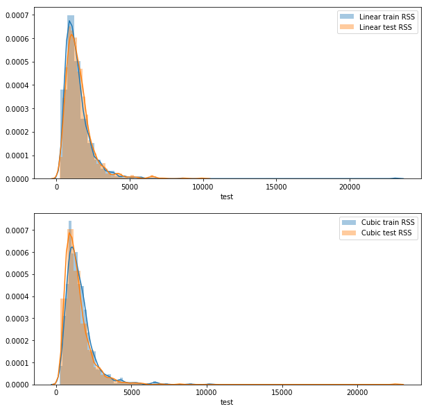
Not what I expected!

• For the linear model, the test RSS is greater than the train RSS
• For the cubic model, the train RSS is greater than the test RSS
• The linear train RSS is less than the cubic train RSS
• The linear test RSS is greater than the cubic test RSS

In light of these results, I don’t know how to answer this question

TODO

• keep prediction results and use sklearn to evaluate performance
• visualize (diagnostic plots) to make sure data is really linear

Exercise 5: The fitted values are linear combinations of the response values.

We have

$\begin{aligned} \hat{y}_i &= x_i\hat{\beta}\\ &= x_i\left(\frac{\sum_{i} x_iy_i}{\sum_{j} x_{i'}^2}\right)\\ &= \frac{1}{\sum_{j} x_{j}^2}\left( x_i \left(\sum_{i} x_iy_i\right)\right)\\ &= \frac{1}{\sum_{j} x_{j}^2}\left(\sum_{i'}x_ix_{i'}y_{i'}\right)\\ &= \sum_{i'}\left(\frac{x_ix_{i'}}{\sum_{j} x_{j}^2}\right)y_{i'}\\ &= \sum_{i'} a_{i'}y_{i'}\\ \end{aligned}$

where

$a_{i'} = \frac{x_ix_{i'}}{\sum_{j} x_{j}^2}$

Exercise 6: Least squares line in simple regression passes through the sample means

Equation (3.4) in the text shows that, in simple regression the coefficients satisfy

$\hat{\beta}_0 = \overline{y} - \hat{\beta}_1\overline{x}$

The least squares line is $y = \hat{\beta}_0 + \hat{\beta}_1 x$, but by 3.4,

$\overline{y} = \hat{\beta}_0 + \hat{\beta}_1 \overline{x}$

which means $(\overline{x}, \overline{y})$ is on the line

Exercise 7: $R^2 = r^2$ ed simple regression

We have

$\begin{aligned} R^2 &= \frac{TSS - RSS}{RSS}\\ &= \frac{\sum_i (y_i - \overline{y})^2 - \sum_i (y_i - \hat{y}_i)^2}{\sum_i (y_i - \overline{y})^2}\\ &= \frac{\sum_i (y_i - \overline{y})^2 - \sum_i (y_i - \hat{\beta}_0 - \hat{\beta}_1 x_i)^2}{\sum_i (y_i - \overline{y})^2}\\ \end{aligned}$

Since

$\begin{aligned} \hat{\beta}_0 = \overline{y} - \hat{\beta}_1\overline{x} \end{aligned}$

The right hand term in the numerator of (3) can be rewritten

$\begin{aligned} \sum_i (y_i - \hat{\beta}_0 - \hat{\beta}_1 x_i)^2 & = \sum_i \left(y_i - \overline{y} - \hat{\beta}_1(x_i - \overline{x})\right)^2 \\ &= \sum_i (y_i - \overline{y})^2 - 2\hat{\beta}_1(y_i - \overline{y})(x_i - \overline{x}) + \hat{\beta}_1^2(x_i - \overline{x})^2\\ \end{aligned}$

substituting (5) into (3) we find

$\begin{aligned} R^2 &= \frac{\sum_i 2\hat{\beta}_1(y_i - \overline{y})(x_i - \overline{x}) - \hat{\beta}_1^2(x_i - \overline{x})^2}{\sum_i (y_i - \overline{y})^2}\\ &= \frac{1}{\sum_i (y_i - \overline{y})^2}\left(2\hat{\beta}_1\left(\sum_i (y_i - \overline{y})(x_i - \overline{x})\right) - \hat{\beta}_1^2\left(\sum_i(x_i - \overline{x})^2\right)\right) \end{aligned}$

Since

$\begin{aligned} \hat{\beta}_1 &= \frac{\sum_j (x_j - \overline{x})(y_j - \overline{y})}{\sum_j(x_j - \overline{x})^2} \end{aligned}$

We can substitute (7) into (6) to get

$\begin{aligned} R^2 &= \frac{1}{\sum_i (y_i - \overline{y})^2}\left(2\left(\left(\frac{\sum_j (x_j - \overline{x})(y_j - \overline{y})}{\sum_j(x_j - \overline{x})^2}\right)\sum_i (y_i - \overline{y})(x_i - \overline{x})\right) - \left(\frac{\sum_j (x_j - \overline{x})(y_j - \overline{y})}{\sum_j(x_j - \overline{x})^2}\right)^2\left(\sum_i(x_i - \overline{x})^2\right)\right)\\ &= \frac{1}{\sum_i (y_i - \overline{y})^2 \sum_j(x_j - \overline{x})^2}\left(2\left(\sum_i\sum_j (x_j - \overline{x})(y_j - \overline{y})(y_i - \overline{y})(x_i - \overline{x})\right) - \sum_i\sum_j (x_j - \overline{x})(y_j - \overline{y})(y_i - \overline{y})(x_i - \overline{x})\right)\\ &= \frac{\sum_i\sum_j(x_i - \overline{x})(y_i - \overline{y})(x_j - \overline{x})(y_j - \overline{y})}{\sum_i (x_i - \overline{x})^2\sum_i (y_i - \overline{y})^2}\\ &= \left(\frac{\sum_i(x_i - \overline{x})(y_i - \overline{y})}{\sqrt{\sum_i (x_i - \overline{x})^2}\sqrt{\sum_i (y_i - \overline{y})^2}}\right)^2\\ &= r^2 \end{aligned}$